What Is the Nearest Positive Semidefinite Matrix?

Given a symmetric matrix and a nonnegative number $\delta$ , what is the nearest symmetric matrix whose eigenvalues are all at least $\delta$ ? In other words, how can we project a symmetric matrix onto the set of symmetric positive semidefinite matrices with eigenvalues at least $\delta$ ?

Distance can be measured in any norm, but the most common choice is the Frobenius norm, $\|A\|_F = (\sum_{i,j = 1}^n |a_{ij}|^2)^{1/2}$ .

This problem occurs in a very wide range of applications. A typical scenario is that a covariance matrix is approximated in some way that does not guarantee positive semidefinitess, for example by treating blocks of the matrix independently. In machine learning, some methods use indefinite kernels and these can require an indefinite similarity matrix to be replaced by a semidefinite one. When $\delta > 0$ , the problem arises when the matrix is positive definite but ill conditioned and a matrix of smaller condition number is required, or when rounding errors result in small negative eigenvalues and a “safely positive definite” matrix is wanted.

The following theorem gives the solution to the problem for the Frobenius norm.

Theorem (Cheng and Higham, 1998).

Let the symmetric matrix $A\in\mathbb{R}^{n \times n}$ have the spectral decomposition $A = Q \mskip1mu\mathrm{diag}(\lambda_i) \mskip1muQ^T$ and let $\delta \ge 0$ . The unique matrix with smallest eigenvalue at least $\delta$ nearest to $A$ in the Frobenius norm is given by

$\notag X = Q \mskip1mu \mathrm{diag}(\tau_i) \mskip1mu Q^T, \quad \tau_i = \begin{cases} \lambda_i, & \lambda_i \geq \delta\\ \delta, & \lambda_i < \delta. \end{cases}$

The theorem says that there is a unique nearest matrix and that is has the same eigenvectors as $A$ with any eigenvalues less than $\delta$ increased to $\delta$ . When $\delta = 0$ , another way to express this result is in terms of the polar decomposition $A = UH$ , where $U$ is orthogonal and $H$ is symmetric positive definite (with $H = Q \mskip1mu\mathrm{diag}(|\lambda_i|)Q^T$ , since $A$ is symmetric): $X = (A + H)/2$ .

One can pose the same nearness problem for nonsymmetric $A$ . For the Frobenius norm there is again a unique nearest symmetric matrix whose eigenvalues are all at least $\delta$ , and it is given by applying the theorem to the symmetric part $B$ of $A$ (which is the nearest symmetric matrix to $A$ ), where

$\notag A = \frac{1}{2} (A + A^T ) + \frac{1}{2} (A - A^T ) \equiv B + C, \quad(B = B^T, ~C = -C^T).$

For the $2$ -norm the answer is known for nonsymmetric $A$ only for $\delta = 0$ , so we take $\delta = 0$ from this point on. We write $X \ge 0$ to denote that the symmetric matrix $X$ is positive semidefinite and use a superscript $1/2$ to denote the positive semidefinite square root.

Theorem (Halmos, 1972).

The $2$ -norm distance from $A\in\mathbb{R}^{n \times n}$ to the nearest positive semidefinite matrix is

$\notag d_2(A) = \min\{\, r \ge 0: r^2I + C^2 \ge 0 ~\mathrm{and}~ G(r) \ge 0 \,\},$

where

$\notag G(r) = B + \bigl(r^2I + C^2\bigr)^{1/2},$

and a nearest matrix is

$\notag X = B + (d_2(A)^2I + C^2)^{1/2}.$

When $A$ is symmetric, so that $C = 0$ , the nearest matrix and the distance reduce to

$\notag X = B + d_2(A)I, \quad d_2(A) = \max\{\, |\lambda_i| : \lambda_i < 0 \,\}.$

Clearly, $X$ is not, in general, unique because when $A$ is symmetric, instead of shifting $B$ by a multiple of $I$ we could just perturb the negative eigenvalue to zero, as with the optimal Frobenius norm perturbation, without changing the $2$ -norm of the perturbation. A distinguishing feature of $X$ in Halmos’s theorem is that $X-P \ge 0$ for any other nearest positive semidefinite matrix $P$ (Bouldin, 1973, Theorem 4.2); thus $X$ has the minimum number of zero eigenvalues over all nearest positive semidefinite matrices.

The Frobenius norm solution $X_F$ is an approximate minimizer of the $2$ -norm distance since (Higham, 1988)

$\notag d_2(A) \le \| A - X_F \|_F \le 2 d_2(A).$

Halmos’s theorem simplifies the computation of $d_2(A)$ because it reduces the minimization problem to one dimension. However, the problem is nonlinear and has no closed form solution for general $A$ , so iterative methods are needed to compute $d_2(A)$ . Two algorithms are developed in Higham (1988). Both are based on the following properties of the matrix $G(r)$ in the theorem: $\lambda_{\min}(G(r))$ is monotone increasing on $[\,\rho(C), \infty)$ , and either $\lambda_{\min}(G(\rho(C))) \ge 0$ , in which case $d_2(A) = \rho(C)$ , or $\lambda_{\min}(G(r))$ has a unique zero $r^* = d_2(A) > \rho(C)$ . The first algorithm uses the bisection method, determining the sign of $\lambda_{\min}(G(r))$ by attempting a Cholesky factorization of $G(r)$ : the sign is nonnegative if the factorization exists and negative otherwise. This approach is attractive if $d_2(A)$ is required only to low accuracy. For higher accuracy computations it is better to apply a more rapidly converging zero finder to $f(r) = \lambda_{\min} (G(r)) = 0$ . A hybrid Newton–bisection method is used in Higham (1988).

Example

For a numerical example (in MATLAB), we take the Jordan block

$\notag A = \begin{bmatrix} 0 & 1 & 0 & 0 & 0 \\ 0 & 0 & 1 & 0 & 0 \\ 0 & 0 & 0 & 1 & 0 \\ 0 & 0 & 0 & 0 & 1 \\ 0 & 0 & 0 & 0 & 0 \end{bmatrix}.$

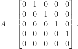
The symmetric part of $A$ , $B = (A+A^T)/2$ , has two negative eigenvalues and a zero eigenvalue:

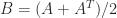
>> A = gallery('jordbloc',5,0); As = sym(A); eig_B = eig((As+As')/2)'
eig_B =
[-1/2, 0, 1/2, -3^(1/2)/2, 3^(1/2)/2]
>> double(eig_B)
ans =
  -5.0000e-01            0   5.0000e-01  -8.6603e-01   8.6603e-01

The nearest symmetric positive semidefinite matrix to $A$ in the Frobenius norm can be computed in MATLAB as

B = (A + A')/2; [Q,D] = eig(B); d = diag(D); X_F = Q*diag(max(d,0))*Q';

We can improve this code by using the implicit expansion feature of MATLAB to avoid forming a diagonal matrix. Since the computed result is not exactly symmetric because of rounding errors, we also need to replace it by the nearest symmetric matrix:

[Q,d] = eig(B,'vector'); X_F = Q*(max(d,0).*Q'); X_F = (X_F + X_F')/2;

We obtain

X_F = 
 1.972e-01   2.500e-01   1.443e-01  -4.163e-17  -5.283e-02  
 2.500e-01   3.415e-01   2.500e-01   9.151e-02  -1.665e-16  
 1.443e-01   2.500e-01   2.887e-01   2.500e-01   1.443e-01  
-4.163e-17   9.151e-02   2.500e-01   3.415e-01   2.500e-01  
-5.283e-02  -1.665e-16   1.443e-01   2.500e-01   1.972e-01

which has eigenvalues

-3.517e-17   7.246e-17   9.519e-17   5.000e-01   8.660e-01

Notice that the three eigenvalues that would be zero in exact arithmetic are of order the unit roundoff. A nearest matrix in the $2$ -norm, as given by Halmos’s theorem. is

X_2 = 
 8.336e-01   5.000e-01   1.711e-01   0.000e+00  -1.756e-02  
 5.000e-01   6.625e-01   5.000e-01   1.887e-01   0.000e+00  
 1.711e-01   5.000e-01   6.450e-01   5.000e-01   1.711e-01  
 0.000e+00   1.887e-01   5.000e-01   6.625e-01   5.000e-01  
-1.756e-02   0.000e+00   1.711e-01   5.000e-01   8.336e-01

and its eigenvalues are

-7.608e-17   1.281e-01   5.436e-01   1.197e+00   1.769e+00

The distances are

$\notag \begin{aligned} 1.732 &= \|A - X_F\|_F < \|A - X_2\|_F = 2.207,\\ 0.9872 &= \|A - X_2\|_2 < \|A - X_F\|_2 = 1.0355. \end{aligned}$

References

This is a minimal set of references, which contain further useful references within.

Richard Bouldin, Positive Approximants, Trans. Amer. Math. Soc. 177, 391–403, 1973.
Sheung Hun Cheng and Nicholas Higham, A Modified Cholesky Algorithm Based on a Symmetric Indefinite Factorization, SIAM J. Matrix Anal. Appl. 19(4), 1097–1110, 1998.
Nicholas J. Higham, Computing a Nearest Symmetric Positive Semidefinite Matrix, Linear Algebra Appl. 103, 103-118, 1988
Paul R. Halmos, Positive Approximants of Operators, Indiana Univ. Math. J. 21, 951–960, 1972.

What Is the Nearest Positive Semidefinite Matrix?

Example

References

Related Blog Posts

Leave a comment Cancel reply

Example

References

Related Blog Posts

Share this:

Related

Leave a comment Cancel reply