For an 

with nonsingular 


More generally, for an index vector ![\alpha = [i_1,i_2,\dots,i_k]](https://s0.wp.com/latex.php?latex=%5Calpha+%3D+%5Bi_1%2Ci_2%2C%5Cdots%2Ci_k%5D&bg=ffffff&fg=222222&s=0&c=20201002)


Schur Complements in Gaussian Elimination
The reduced submatrices in Gaussian elimination are Schur complements. Write an
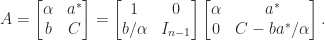
This factorization represents the first step of Gaussian elimination.
After 

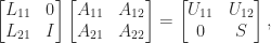
where the first matrix on the left is the product of the elementary transformations that reduce the first 


The next step of the elimination, which zeros out the first column of 

For a number of matrix structures, such as
- Hermitian (or real symmetric) positive definite matrices,
- totally positive matrices,
- matrices diagonally dominant by rows or columns,
-matrices,
one can show that the Schur complement inherits the structure. For these four structures the
Inverse of a Block Matrix
The Schur complement arises in formulas for the inverse of a block 

If
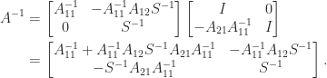
So 

One can obtain an analogous formula for 
Test for Positive Definiteness
For Hermitian matrices the Schur complement provides a test for positive definiteness. Suppose
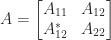
with

shows that 
Generalized Schur Complement
For 
Theorem 1.
If
is Hermitian then
and
are both positive semidefinite.

If
Notes and References
The term “Schur complement” was coined by Haynsworth in 1968, thereby focusing attention on this important form of matrix and spurring many subsequent papers that explore its properties and applications. The name “Schur” was chosen because a 1917 determinant lemma of Schur says that if

which is obtained by taking determinants in (2).
For much more about the Schur complement see Zhang (2005) or Horn and Johnson (2013).
- Emilie V. Haynsworth, Determination of the Inertia of a Partitioned Matrix, Linear Algebra Appl. 1(1), 73–81, 1968.
- Roger A. Horn and Charles R. Johnson, Matrix Analysis, second edition, Cambridge University Press, 2013. My review of the second edition.
- Fuzhen Zhang, editor, The Schur Complement and Its Applications. Springer-Verlag, New York, 2005, xvi+295 pp.
Related Blog Posts
- What Is a Block Matrix? (2020)
- What is a Diagonally Dominant Matrix? (2021)
- What Is a Symmetric Positive Definite Matrix? (2020)
- What Is a Totally Nonnegative Matrix? (2021)
- What Is an LU Factorization? (2021)
- What Is an M-Matrix? (2021)
- What Is the Inertia of a Matrix? (2022)
- What Is the Matrix Inverse? (2022)
This article is part of the “What Is” series, available from https://nhigham.com/category/what-is and in PDF form from the GitHub repository https://github.com/higham/what-is.

 for all
  at
at  is
is
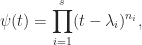
 ). The polynomial
  .
.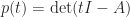 , a degree
  monic polynomial whose roots are the eigenvalues of
  , but
, but  may not be the polynomial of lowest degree that annihilates
  of lowest degree such that
  is the minimal polynomial of
  , and in particular it divides the characteristic polynomial. Indeed by polynomial long division we can write
 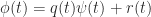 , where the degree of
  is less than the degree of
 then we have a contradiction to the minimality of the degree of
  and so
  and
and  are two different monic polynomials of minimum degree
  such that
  ,
,  , then
  is a polynomial of degree less than
  , and we can scale
  to be monic, so by the minimality of
  , or
, or  .
. , since
  . On the other hand, for the Jordan block
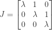
 .
.
 are the distinct eigenvalues of
  is the dimension of the largest Jordan block in which
  appears. This expression is composed of linear factors (that is,
  for all
  ) if and only if
 ![\notag A = \left[\begin{array}{cc|c|c|c} \lambda & 1 & & & \\ & \lambda & & & \\\hline & & \lambda & & \\\hline & & & \mu & \\\hline & & & & \mu \end{array}\right]](https://s0.wp.com/latex.php?latex=%5Cnotag++A+%3D+%5Cleft%5B%5Cbegin%7Barray%7D%7Bcc%7Cc%7Cc%7Cc%7D++++++%5Clambda+%26++1++++++%26+++++++++%26+++++%26+++%5C%5C++++++++++++++%26+%5Clambda+%26+++++++++%26+++++%26+++%5C%5C%5Chline++++++++++++++%26+++++++++%26+%5Clambda+%26+++++%26+++%5C%5C%5Chline++++++++++++++%26+++++++++%26+++++++++%26+%5Cmu+%26++++%5C%5C%5Chline++++++++++++++%26+++++++++%26+++++++++%26+++++%26+%5Cmu+++%5Cend%7Barray%7D%5Cright%5D+&bg=ffffff&fg=222222&s=0&c=20201002)
 , while the characteristic polynomial is
  .
. matrix,
  ? Since
  , we have
  for
for  . For any linear polynomial
  ,
,  , which is nonzero since
  has rank
  has rank
  .
.
 to a linear system of equations
  , where
  .
. .
. .
. (where we include the permutations in
  ). Most of the work is in the LU factorization, which costs
  flops, and each iteration requires a multiplication with
  , which total only
  flops. If the refinement converges quickly then it is inexpensive.
 satisfies (omitting constants)
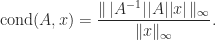
 is the matrix condition number in the
  -norm. We would like refinement to produce a solution accurate to precision
 .
. to the level of
  , the unit roundoff for IEEE single precision arithmetic.
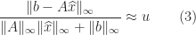

 is no larger than
  and can be much smaller, especially if
  by substitution in single precision, obtaining
  in single precision.
 entirely in double precision arithmetic. The algorithm achieves the same limiting accuracy (4) and limiting residual (3) provided that
  .
.
 is not formed but is applied to a vector as a multiplication with
  . As long as GMRES converges quickly for this preconditioned system the speed again from the fast single precision factorization will not be lost. Moreover, this different step 4 results in convergence for
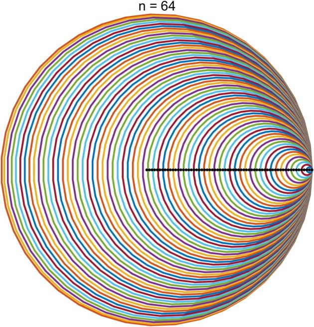

 is to
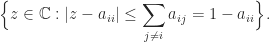
is to  containing all the others.
![[0,1]](https://s0.wp.com/latex.php?latex=%5B0%2C1%5D&bg=ffffff&fg=222222&s=0&c=20201002) , so the centers of the discs are roughly equally spaced and shrink as the centers move to the right.
, so the centers of the discs are roughly equally spaced and shrink as the centers move to the right. . The black dots are the eigenvalues. Here is the plot for
  . The function used to produce these plots is
  Here are two other matrices whose Gershgorin discs make a graphically interesting plot.

 . The trace is linear, that is,
  , and
, and  .
. . The roots of
  of
of 
 . The Laplace expansion of
  shows that the coefficient of
  is
is  . Equating these two expressions for
  gives
gives
 for any nonsingular
  .
. . If there are
  then
then  and
and  . Therefore
  and
and  .
. matrix
  matrix
  ,
,
 in general). The proof is simple:
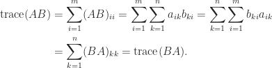
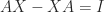 in
in  , which is a contradiction. Therefore the equation has no solution.
 for
for  , that is,
 and
and  are
are  . If
. If  can be evaluated without forming the matrix
  since, by (3),
  .
.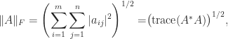
 denotes the conjugate transpose. For example, we can generalize the formula
 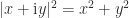 for a complex number to an
 and
and  . Then
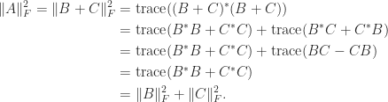
 and variance
 for
for  and
and  for all
  . This stochastic estimate, which is due to Hutchinson, is therefore unbiased.
 is diagonalizable if there exists a nonsingular matrix
  such that
  is diagonal. In other words, a diagonalizable matrix is one that is similar to a diagonal matrix.
 is equivalent to
  with
with  ,
,  , where
 ![X = [x_1,x_2,\dots, x_n]](https://s0.wp.com/latex.php?latex=X+%3D+%5Bx_1%2Cx_2%2C%5Cdots%2C+x_n%5D&bg=ffffff&fg=222222&s=0&c=20201002) . Hence
. Hence  ). A matrix with distinct eigenvalues is also diagonalizable.
 has distinct eigenvalues then it is diagonalizable.
 with corresponding eigenvectors
  . Suppose that
  for some
  . Then
 since
since  for
for  and
and  . Premultiplying
  by
by  shows, in the same way, that
  . Continuing in this way we find that
  . Therefore the
  are linearly independent and hence
 ![\bigl[\begin{smallmatrix} 0 & 1 \\ 0 & 0 \end{smallmatrix}\bigr]](https://s0.wp.com/latex.php?latex=%5Cbigl%5B%5Cbegin%7Bsmallmatrix%7D+0+%26+1+%5C%5C+0+%26+0+%5Cend%7Bsmallmatrix%7D%5Cbigr%5D&bg=ffffff&fg=222222&s=0&c=20201002) . This matrix is a
. This matrix is a  .
. , that is, any matrix in
  diagonalizable, where
  are nonzero? There are
  zero eigenvalues with eigenvectors any set of linearly independent vectors orthogonal to
  then
then  is the remaining eigenvalue, with eigenvector
  then all the eigenvalues of
 ![x = \bigl[{1 \atop 0} \bigr]](https://s0.wp.com/latex.php?latex=x+%3D+%5Cbigl%5B%7B1+%5Catop+0%7D+%5Cbigr%5D&bg=ffffff&fg=222222&s=0&c=20201002) and
and ![y = \bigl[{0 \atop 1} \bigr]](https://s0.wp.com/latex.php?latex=y+%3D+%5Cbigl%5B%7B0+%5Catop+1%7D+%5Cbigr%5D&bg=ffffff&fg=222222&s=0&c=20201002) , so
, so 
 is stochastic then
  , where
 ![e = [1,1,\dots,1]^T](https://s0.wp.com/latex.php?latex=e+%3D+%5B1%2C1%2C%5Cdots%2C1%5D%5ET&bg=ffffff&fg=222222&s=0&c=20201002) is the vector of ones. This means that
is the vector of ones. This means that  is an eigenvector of
 ![\notag \begin{aligned} A_n &= n^{-1}ee^T, \quad \textrm{in particular}~~ A_3 = \begin{bmatrix} \frac{1}{3} & \frac{1}{3} & \frac{1}{3}\\[3pt] \frac{1}{3} & \frac{1}{3} & \frac{1}{3}\\[3pt] \frac{1}{3} & \frac{1}{3} & \frac{1}{3} \end{bmatrix}, \qquad (1)\\ B_n &= \frac{1}{n-1}(ee^T -I), \quad \textrm{in particular}~~ B_3 = \begin{bmatrix} 0 & \frac{1}{2} & \frac{1}{2}\\[2pt] \frac{1}{2} & 0 & \frac{1}{2}\\[2pt] \frac{1}{2} & \frac{1}{2} & 0 \end{bmatrix}, \qquad (2)\\ C_n &= \begin{bmatrix} 1 & & & \\ \frac{1}{2} & \frac{1}{2} & & \\ \vdots & \vdots &\ddots & \\ \frac{1}{n} & \frac{1}{n} &\cdots & \frac{1}{n} \end{bmatrix}. \qquad (3)\\ \end{aligned}](https://s0.wp.com/latex.php?latex=%5Cnotag+%5Cbegin%7Baligned%7D+++A_n+%26%3D+n%5E%7B-1%7Dee%5ET%2C+%5Cquad+%5Ctextrm%7Bin+particular%7D%7E%7E+++++A_3+%3D+%5Cbegin%7Bbmatrix%7D++++%5Cfrac%7B1%7D%7B3%7D+%26+%5Cfrac%7B1%7D%7B3%7D+%26+%5Cfrac%7B1%7D%7B3%7D%5C%5C%5B3pt%5D++++%5Cfrac%7B1%7D%7B3%7D+%26+%5Cfrac%7B1%7D%7B3%7D+%26+%5Cfrac%7B1%7D%7B3%7D%5C%5C%5B3pt%5D++++%5Cfrac%7B1%7D%7B3%7D+%26+%5Cfrac%7B1%7D%7B3%7D+%26+%5Cfrac%7B1%7D%7B3%7D++++%5Cend%7Bbmatrix%7D%2C+%5Cqquad+%281%29%5C%5C+++B_n+%26%3D+%5Cfrac%7B1%7D%7Bn-1%7D%28ee%5ET+-I%29%2C+%5Cquad+%5Ctextrm%7Bin+particular%7D%7E%7E+++++B_3+%3D+%5Cbegin%7Bbmatrix%7D++++++++++++++0+%26+%5Cfrac%7B1%7D%7B2%7D+%26+%5Cfrac%7B1%7D%7B2%7D%5C%5C%5B2pt%5D++++%5Cfrac%7B1%7D%7B2%7D+%26+0+++++++++++%26+%5Cfrac%7B1%7D%7B2%7D%5C%5C%5B2pt%5D++++%5Cfrac%7B1%7D%7B2%7D+%26+%5Cfrac%7B1%7D%7B2%7D+%26+0++++%5Cend%7Bbmatrix%7D%2C++++%5Cqquad+%282%29%5C%5C+++C_n+%26%3D+%5Cbegin%7Bbmatrix%7D+++++++++++++1+++++++++%26+++++++++++++++++++%26+++++++++++%26++++%5C%5C++++++%5Cfrac%7B1%7D%7B2%7D++++++%26++%5Cfrac%7B1%7D%7B2%7D++++++%26+++++++++++%26++++%5C%5C++++++%5Cvdots+++++++++++%26++%5Cvdots+++++++++++%26%5Cddots+++++%26++++%5C%5C++++++%5Cfrac%7B1%7D%7Bn%7D++++++%26++%5Cfrac%7B1%7D%7Bn%7D++++++%26%5Ccdots+++++%26++%5Cfrac%7B1%7D%7Bn%7D++++++%5Cend%7Bbmatrix%7D.+++%5Cqquad+%283%29%5C%5C+%5Cend%7Baligned%7D+&bg=ffffff&fg=222222&s=0&c=20201002)
 is bounded by
  for any norm. For a stochastic matrix, taking the
  , so since we know that
  . It can be shown that
  , which implies
  . Every eigenvalue
  lies in the union of the
 is nonnegative and
  , so
, so  converge as
  ? The answer is that it does, and the limit is stochastic, as long as
 , all even powers are equal to
  for all
  as
as  converges to the matrix with
  element is the probability of moving from state
  over a time step. It has nonnegative entries and the rows sum to
  , is a transition matrix for a time period a factor
  (years to months) and
  (weeks to days) are among the values of interest. Unfortunately, a stochastic

 (so that
  is row-stochastic). A matrix that is both row-stochastic and column-stochastic is called doubly stochastic. A permutation matrix is an example of a doubly stochastic matrix. If
  is doubly stochastic. A magic square scaled by the magic sum is also doubly stochastic. For example,
 , where
  is the number of positive eigenvalues of
  is the number of negative eigenvalues of
  is the number of zero eigenvalues of
  . The difference
  is called the signature.
 and
and  . But in general the diagonal elements do not tell us much about the inertia. For example, here is a matrix that has positive diagonal elements but only one positive eigenvalue (and this example works for any
  for a nonsingular matrix
  is nonsingular then
  .
. does the job, where
  is a permutation matrix,
  is diagonal Then
  , and
, and  can be read off the diagonal of
  factorization, in which
  , always exists, and its computation is numerically stable with a suitable pivoting strategy such as symmetric rook pivoting.
 .
. and
and 
 .
.