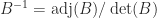
The Cayley–Hamilton Theorem says that a square matrix 


and the Cayley–Hamilton theorem says that

Various proofs of the theorem are available, of which we give two. The first is the most natural for anyone familiar with the Jordan canonical form. The second is more elementary but less obvious.
First proof.
Consider a 

We have
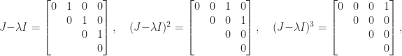
and then 


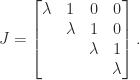
Let 


and 

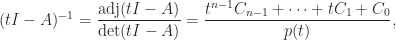
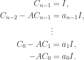
Second Proof
Recall that the adjugate 


for some matrices 


and equating coefficients of 

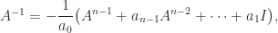
Premultiplying the first equation by 


as required. This proof is by Buchheim (1884).
Applications and Generalizations
A common use of the Cayley–Hamilton theorem is to show that 

since 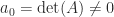
Similarly, 


where 
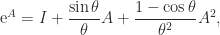
Cayley used the Cayley–Hamilton theorem to find square roots of a 


which gives

Now 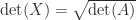


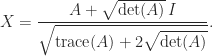
With appropriate choices of signs for the square roots this formula gives all four square roots of
Expressions obtained from the Cayley–Hamilton theorem are of little practical use for general matrices, because algorithms that compute the coefficients 
The Cayley–Hamilton theorem has been generalized in various directions. The theorem can be interpreted as saying that the powers 


Historical Note
The Cayley–Hamilton theorem appears in the 1858 memoir in which Cayley introduced matrix algebra. Cayley gave a proof for 


References
- Arthur Buchheim, Mathematical Notes, Messenger Math. 13, 62–66, 1884.
- Arthur Cayley, A Memoir on the Theory of Matrices, Philos. Trans. Roy. Soc. London 148, 17–37, 1858.
- Tony Crilly, Cayley’s Anticipation of a Generalised Cayley–Hamilton Theorem, Historia Mathematica 5, 211–219, 1978.
Related Blog Posts
- What Is the Adjugate of a Matrix? (2020)
- What Is the Gerstenhaber Problem? (2020)
- What Is the Matrix Exponential? (2020)
- What Is the Square Root of a Matrix? (2020)
This article is part of the “What Is” series, available from https://nhigham.com/category/what-is and in PDF form from the GitHub repository https://github.com/higham/what-is.
