What Is an Eigenvalue?

An eigenvalue of a square matrix A is a scalar \lambda such that Ax = \lambda x for some nonzero vector x. The vector x is an eigenvector of A and it has the distinction of being a direction that is not changed on multiplication by A.

An n\times n matrix has n eigenvalues. This can be seen by noting that Ax = \lambda x is equivalent to (\lambda I - A) x = 0, which means that \lambda I - A is singular, since x\ne 0. Hence \det(\lambda I - A) = 0. But

\notag  \det(\lambda I - A) = \lambda^n +                        a_{n-1}\lambda^{n-1} + \cdots + a_1 \lambda + a_0

is a scalar polynomial of degree n (the characteristic polynomial of A) with nonzero leading coefficient and so has n roots, which are the eigenvalues of A. Since \det(\lambda I - A) = \det( (\lambda I - A)^T)       = \det(\lambda I - A^T), the eigenvalues of A^T are the same as those of A.

A real matrix may have complex eigenvalues, but they appear in complex conjugate pairs. Indeed Ax = \lambda x implies \overline{A}\overline{x} = \overline{\lambda} \overline{x}, so if A is real then \overline{\lambda} is an eigenvalue of A with eigenvector \overline{x}.

Here are some 2\times 2 matrices and their eigenvalues.

\notag \begin{aligned}  A_1 &= \begin{bmatrix}1 & 0 \\ 0 & 1 \end{bmatrix}, \quad         \lambda = 1,1,\\  A_2 &= \begin{bmatrix}0 & 1 \\ 0 & 0 \end{bmatrix}, \quad         \lambda = 0,0,\\  A_3 &= \begin{bmatrix}0 & 1 \\ -1 & 0 \end{bmatrix}, \quad         \lambda = \mathrm{i},\mathrm{-i}. \end{aligned}

Note that A_1 and A_2 are upper triangular, that is, a_{ij} = 0 for i>j. For such a matrix the eigenvalues are the diagonal elements.

A symmetric matrix (A^T = A) or Hermitian matrix (A^* = A, where A^* = \overline{A}^T) has real eigenvalues. A proof is Ax = \lambda x \Rightarrow x^*A^* = \overline{\lambda} x^* so premultiplying the first equation by x^* and postmultiplying the second by x gives x^*Ax = \lambda x^*x and x^*Ax = \overline{\lambda} x^*x, which means that (\lambda-\overline{\lambda})x^*x = 0, or \lambda=\overline{\lambda} since x^*x \ne 0. The matrix A_1 above is symmetric.

A skew-symmetric matrix (A^T = -A) or skew-Hermitian complex matrix (A^* = -A) has pure imaginary eigenvalues. A proof is similar to the Hermitian case: Ax = \lambda x \Rightarrow -x^*A = x^*A^* = \overline{\lambda} x^* and so x^*Ax is equal to both \lambda x^*x and -\overline{\lambda} x^*x, so \lambda = -\overline{\lambda}. The matrix A_3 above is skew-symmetric.

In general, the eigenvalues of a matrix A can lie anywhere in the complex plane, subject to restrictions based on matrix structure such as symmetry or skew-symmetry, but they are restricted to the disc centered at the origin with radius \|A\|, because for any matrix norm \|\cdot\| it can be shown that every eigenvalue satisfies |\lambda| \le \|A\|.

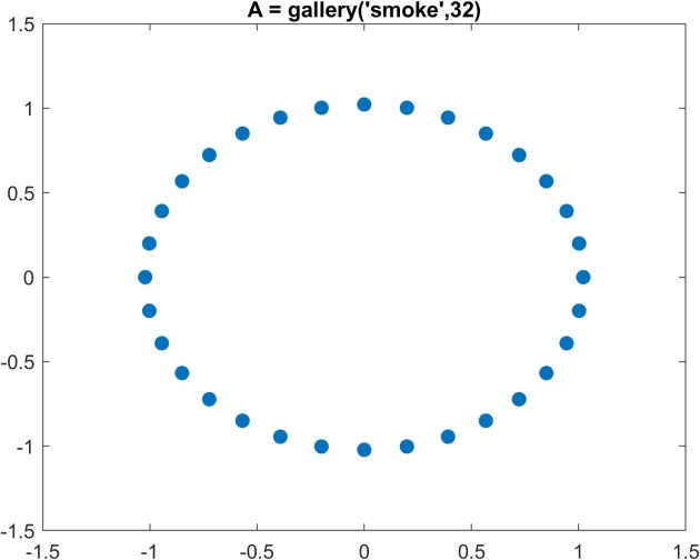
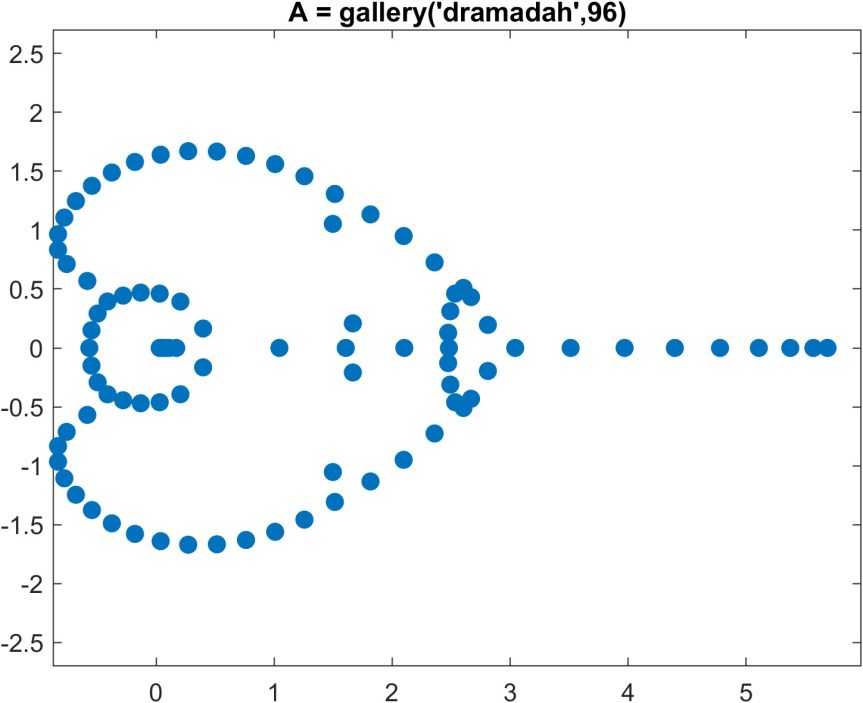
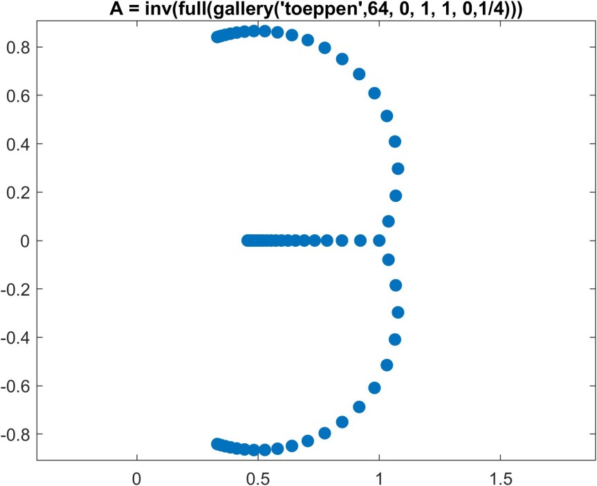
Here are some example eigenvalue distributions, computed in MATLAB. (The eigenvalues are computed at high precision using the Advanpix Multiprecision Computing Toolbox in order to ensure that rounding errors do not affect the plots.) The second and third matrices are real, so the eigenvalues are symmetrically distributed about the real axis. (The first matrix is complex.)

eig_smoke.jpg eig_dramadah.jpg eig_toeppen_inv.jpg

Although this article is about eigenvalues we need to say a little more about eigenvectors. An n\times n matrix A with distinct eigenvalues has n linearly independent eigenvectors. Indeed it is diagonalizable: A = XDX^{-1} for some nonsingular matrix X with D = \mathrm{diag}(\lambda_i) the matrix of eigenvalues. If we write X in terms of its columns as X = [x_1,x_2,\dots,x_n] then AX = XD is equivalent to Ax_i = \lambda _i x_i, i=1\colon n, so the x_i are eigenvectors of A. The matrices A_1 and A_3 above both have two linearly independent eigenvectors.

If there are repeated eigenvalues there can be less than n linearly independent eigenvectors. The matrix A_2 above has only one eigenvector: the vector \left[\begin{smallmatrix}1 \\ 0 \end{smallmatrix}\right] (or any nonzero scalar multiple of it). This matrix is a Jordan block. The matrix A_1 shows that a matrix with repeated eigenvalues can have linearly independent eigenvectors.

Here are some questions about eigenvalues.

  • What matrix decompositions reveal eigenvalues? The answer is the Jordan canonical form and the Schur decomposition. The Jordan canonical form shows how many linearly independent eigenvectors are associated with each eigenvalue.
  • Can we obtain better bounds on where eigenvalues lie in the complex plane? Many results are available, of which the most well-known is Gershgorin’s theorem.
  • How can we compute eigenvalues? Various methods are available. The QR algorithm is widely used and is applicable to all types of eigenvalue problems.

Finally, we note that the concept of eigenvalue is more general than just for matrices: it extends to nonlinear operators on finite or infinite dimensional spaces.

References

Many books include treatments of eigenvalues of matrices. We give just three examples.

  • Gene Golub and Charles F. Van Loan, Matrix Computations, fourth edition, Johns Hopkins University Press, Baltimore, MD, USA, 2013.
  • Roger A. Horn and Charles R. Johnson, Matrix Analysis, second edition, Cambridge University Press, 2013. My review of the second edition.
  • Carl D. Meyer, Matrix Analysis and Applied Linear Algebra, Society for Industrial and Applied Mathematics, Philadelphia, PA, USA, 2000.

Related Blog Posts

This article is part of the “What Is” series, available from https://nhigham.com/category/what-is and in PDF form from the GitHub repository https://github.com/higham/what-is.

Leave a comment