What Is a Permutation Matrix?

A permutation matrix is a square matrix in which every row and every column contains a single $1$ and all the other elements are zero. Such a matrix, $P$ say, is orthogonal, that is, $P^TP = PP^T = I_n$ , so it is nonsingular and has determinant $\pm 1$ . The total number of $n\times n$ permutation matrices is $n!$ .

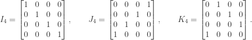
Premultiplying a matrix by $P$ reorders the rows and postmultiplying by $P$ reorders the columns. A permutation matrix $P$ that has the desired reordering effect is constructed by doing the same operations on the identity matrix.

Examples of permutation matrices are the identity matrix $I_n$ , the reverse identity matrix $J_n$ , and the shift matrix $K_n$ (also called the cyclic permutation matrix), illustrated for $n = 4$ by

$\notag I_4 = \begin{bmatrix} 1 & 0 & 0 & 0 \\ 0 & 1 & 0 & 0 \\ 0 & 0 & 1 & 0 \\ 0 & 0 & 0 & 1 \end{bmatrix}, \qquad J_4 = \begin{bmatrix} 0 & 0 & 0 & 1 \\ 0 & 0 & 1 & 0 \\ 0 & 1 & 0 & 0 \\ 1 & 0 & 0 & 0 \end{bmatrix}, \qquad K_4 = \begin{bmatrix} 0 & 1 & 0 & 0 \\ 0 & 0 & 1 & 0 \\ 0 & 0 & 0 & 1 \\ 1 & 0 & 0 & 0 \end{bmatrix}.$

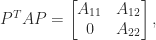
Pre- or postmultiplying a matrix by $J_n$ reverses the order of the rows and columns, respectively. Pre- or postmultiplying a matrix by $K_n$ shifts the rows or columns, respectively, one place forward and moves the first one to the last position—that is, it cyclically permutes the rows or columns. Note that $J_n$ is a symmetric Hankel matrix and $K_n$ is a circulant matrix.

An elementary permutation matrix $P$ differs from $I_n$ in just two rows and columns, $i$ and $j$ , say. It can be written $P = I_n - (e_i-e_j)(e_i-e_j)^T$ , where $e_i$ is the $i$ th column of $I_n$ . Such a matrix is symmetric and so satisfies $P^2 = I_n$ , and it has determinant $-1$ . A general permutation matrix can be written as a product of elementary permutation matrices $P = P_1P_2\dots P_k$ , where $k$ is such that $\det(P) = (-1)^k$ .

It is easy to show that 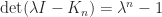$\det(\lambda I - K_n) = \lambda^n - 1$ , which means that the eigenvalues of $K_n$ are $1, w, w^2, \dots, w^{n-1}$ , where $w = \exp(2\pi\mathrm{i}/n)$ is the $n$ th root of unity. The matrix $K_n$ has two diagonals of $1$ s, which move up through the matrix as it is powered: $K_n^i \ne I$ for $i< n$ and $K_n^n = I$ . The following animated gif superposes MATLAB spy plots of $K_{64}$ , $K_{64}^2$ , …, $K_{64}^{64} = I_{64}$ .

The shift matrix $K_n$ plays a fundamental role in characterizing irreducible permutation matrices. Recall that a matrix $A\in\mathbb{C}^{n\times n}$ is irreducible if there does not exist a permutation matrix $P$ such that

$\notag P^TAP = \begin{bmatrix} A_{11} & A_{12} \\ 0 & A_{22} \end{bmatrix},$

where $A_{11}$ and $A_{22}$ are square, nonempty submatrices.

Theorem 1. For a permutation matrix $P \in \mathbb{R}^{n \times n}$ the following conditions are equivalent.

$P$ is irreducible.

There exists a permutation matrix $Q$ such that $Q^{-1}PQ = K_n$

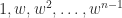
The eigenvalues of $P$ are $1, w, w^2, \dots, w^{n-1}$ .

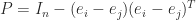
One consequence of Theorem 1 is that for any irreducible permutation matrix $P$ , $\mathrm{rank}(P - I) = \mathrm{rank}(K_n - I) = n-1$ .

The next result shows that a reducible permutation matrix can be expressed in terms of irreducible permutation matrices.

Theorem 2. Every reducible permutation matrix is permutation similar to a direct sum of irreducible permutation matrices.

Another notable permutation matrix is the vec-permutation matrix, which relates $A\otimes B$ to $B\otimes A$ , where $\otimes$ is the Kronecker product.

A permutation matrix is an example of a doubly stochastic matrix: a nonnegative matrix whose row and column sums are all equal to $1$ . A classic result characterizes doubly stochastic matrices in terms of permutation matrices.

Theorem 3 (Birkhoff). A matrix is doubly stochastic if and only if it is a convex combination of permutation matrices.

In coding, memory can be saved by representing a permutation matrix $P$ as an integer vector $p$ , where $p_i$ is the column index of the $1$ within the $i$ th row of $P$ . MATLAB functions that return permutation matrices can also return the permutation in vector form. Here is an example with the MATLAB lu function that illustrates how permuting a matrix can be done using the vector permutation representation.

>> A = gallery('frank',4), [L,U,P] = lu(A); P
A =
     4     3     2     1
     3     3     2     1
     0     2     2     1
     0     0     1     1
P =
     1     0     0     0
     0     0     1     0
     0     0     0     1
     0     1     0     0
>> P*A
ans =
     4     3     2     1
     0     2     2     1
     0     0     1     1
     3     3     2     1
>> [L,U,p] = lu(A,'vector'); p
p =
     1     3     4     2
>> A(p,:)
ans =
     4     3     2     1
     0     2     2     1
     0     0     1     1
     3     3     2     1

For more on handling permutations in MATLAB see section 24.3 of MATLAB Guide.

Notes

For proofs of Theorems 1–3 see Zhang (2011, Sec. 5.6). Theorem 3 is also proved in Horn and Johnson (2013, Thm. 8.7.2).

Permutations play a key role in the fast Fourier transform and its efficient implementation; see Van Loan (1992).

References

Desmond Higham and Nicholas Higham, MATLAB Guide, third edition, SIAM, 2017.
Roger A. Horn and Charles R. Johnson, Matrix Analysis, second edition, Cambridge University Press, 2013. My review of the second edition.
Charles F. Van Loan, Computational Frameworks for the Fast Fourier Transform, SIAM, 1992.
Fuzhen Zhang, Matrix Theory: Basic Results and Techniques, Springer, 2011.

What Is a Permutation Matrix?

Notes

References

Related Blog Posts

Leave a comment Cancel reply

Notes

References

Related Blog Posts

Share this:

Related

Leave a comment Cancel reply