A 


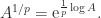
Recall, first, that for a nonzero complex scalar 


Here the logarithm is the principal matrix logarithm, the matrix function built on the principal scalar logarithm, and so the eigenvalues of 
![\alpha \in [-1,1]](https://s0.wp.com/latex.php?latex=%5Calpha+%5Cin+%5B-1%2C1%5D&bg=ffffff&fg=222222&s=0&c=20201002)


The most important special case is 
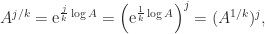
We can check that

so the definition does indeed produce a 
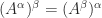
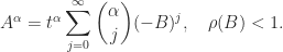
Returning to the case of rational
but 

An integral expression for 
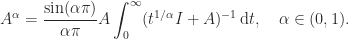
Another representation for 

For 

with 


Computation
The formula 
If 


Inverse Function
If 


Using the matrix unwinding function it can be shown that 


![\alpha\in[-1,1]](https://s0.wp.com/latex.php?latex=%5Calpha%5Cin%5B-1%2C1%5D&bg=ffffff&fg=222222&s=0&c=20201002)
Backward Error
How can we check the quality of an approximation 

For an approximation 

![\notag \eta(X) = \displaystyle\frac{ \|X^{1/\alpha} - A \|}{\|A\|}, \quad \alpha\in[-1,1].](https://s0.wp.com/latex.php?latex=%5Cnotag++++++%5Ceta%28X%29+%3D+%5Cdisplaystyle%5Cfrac%7B+%5C%7CX%5E%7B1%2F%5Calpha%7D+-+A+%5C%7C%7D%7B%5C%7CA%5C%7C%7D%2C+%5Cquad+%5Calpha%5Cin%5B-1%2C1%5D.+&bg=ffffff&fg=222222&s=0&c=20201002)
Applications with Stochastic Matrices
An important application of fractional matrix powers is in discrete-time Markov chains, which arise in areas including finance and medicine. A transition matrix for a Markov process is a matrix whose 


![\notag A = \left[\begin{array}{ccc} 0 & 1 & 0\\ 0 & 0 & 1\\ 1 & 0 & 0\\ \end{array} \right]](https://s0.wp.com/latex.php?latex=%5Cnotag++++A+%3D+%5Cleft%5B%5Cbegin%7Barray%7D%7Bccc%7D++++++++0++%26+1+%26+0%5C%5C++++++++0++%26+0+%26+1%5C%5C++++++++1++%26+0+%26+0%5C%5C++++++++%5Cend%7Barray%7D+%5Cright%5D+&bg=ffffff&fg=222222&s=0&c=20201002)
has principal square root
![\notag A^{1/2} = \frac{1}{3} \left[\begin{array}{rrr} 2 & 2 & -1 \\ -1 & 2 & 2 \\ 2 & -1 & 2 \end{array} \right],](https://s0.wp.com/latex.php?latex=%5Cnotag++++A%5E%7B1%2F2%7D+%3D+%5Cfrac%7B1%7D%7B3%7D+%5Cleft%5B%5Cbegin%7Barray%7D%7Brrr%7D++++++++2++%26+2+%26+-1+%5C%5C++++++++-1+%26+2+%26+2+%5C%5C++++++++2+%26+-1+%26+2++++++++%5Cend%7Barray%7D+%5Cright%5D%2C+&bg=ffffff&fg=222222&s=0&c=20201002)
but 
![\notag Y = \left[\begin{array}{ccc} 0 & 0 & 1\\ 1 & 0 & 0\\ 0 & 1 & 0\\ \end{array} \right]](https://s0.wp.com/latex.php?latex=%5Cnotag+++++++++Y+%3D+%5Cleft%5B%5Cbegin%7Barray%7D%7Bccc%7D++++++++++0++%26+0++%26++1%5C%5C++++++++++1++%26+0++%26++0%5C%5C++++++++++0++%26+1++%26++0%5C%5C++++++++++%5Cend%7Barray%7D+%5Cright%5D+&bg=ffffff&fg=222222&s=0&c=20201002)
is stochastic, though. (Interestingly, 
A wide variety configurations is possible as regards existence, nature (primary or nonprimary), and number of stochastic roots. Higham and Lin (2011) delineate the various possibilities that can arise. They note that the stochastic lower triangular matrix

has a stochastic 

The existence of stochastic roots of stochastic matrices is connected with the embeddability problem, which asks when a nonsingular stochastic matrix 


Applications in Fractional Differential Equations
Fractional matrix powers arise in the numerical solution of differential equations of fractional order, especially partial differential equations involving fractional Laplace operators. Here, the problem may be one of computing 
References
This is a minimal set of references, which contain further useful references within.
- Brian Davies, Embeddable Markov Matrices, Electronic J. Probability 15, 1474–1486, 2010.
- Roberto Garrappa and Marina Popolizio, On the Use of Matrix Functions for Fractional Partial Differential Equations, Math. Comput. Simulation C-25(81), 1045–1056, 2011.
- Nicholas J. Higham, Functions of Matrices: Theory and Computation, Society for Industrial and Applied Mathematics, Philadelphia, PA, USA, 2008.
- Nicholas J. Higham and Lijing Lin, On
- Nicholas Higham and Lijing Lin, An Improved Schur–Padé Algorithm for Fractional Powers of a Matrix and their Fréchet Derivatives, SIAM J. Matrix Anal. Appl. 34(3), 1341–1360, 2013.
- Emmanuel Lorin and Simon Tian, A Numerical Study of Fractional Linear Algebraic Systems, Math. Comput. Simulation 182, 495–513, 2021.
Related Blog Posts
- Update of Catalogue of Software for Matrix Functions (2020)
- What Is a Matrix Function? (2020)
- What Is a Matrix Square Root? (2020)
- What Is the Matrix Exponential? (2020)
- What Is the Matrix Logarithm? (2020)
- What Is the Matrix Unwinding Function? (2020)
This article is part of the “What Is” series, available from https://nhigham.com/category/what-is and in PDF form from the GitHub repository https://github.com/higham/what-is.

The fractional powers of unitary matrices are not unique because of the phase freedom. Does the integral representation take this fact into account? Are there any other constraints on fractional powers of unitary matrices?
A^\alpha as defined here is unique even for unitary matrices: the (principal) log in the definition takes care of phase freedom. So unitary matrices are not special as regards fractional powers.
Dear professor Nick, thank you for your reply. I have been trying to understand the fractional powers of unitaries. I know you had cited a few references in the post. It seems that these references mostly talk about these matrices in a more general sense. It would be nice to see if any other papers/articles that deal with unitary cases rigorously.