What Is the Matrix Sign Function?

The matrix sign function is the matrix function corresponding to the scalar function of a complex variable

$\notag \mathrm{sign}(z) = \begin{cases} 1, & \mathop{\mathrm{Re}} z > 0, \\ -1, & \mathop{\mathrm{Re}} z < 0. \end{cases}$

Note that this function is undefined on the imaginary axis. The matrix sign function can be obtained from the Jordan canonical form definition of a matrix function: if $A = XJX^{-1}$ is a Jordan decomposition with $\mathrm{diag}(J) = \mathrm{diag}(\lambda_i)$ then

$\notag S = \mathrm{sign}(A) = X \mathrm{sign}(J)X^{-1} = X \mathrm{diag}(\mathrm{sign}(\lambda_i))X^{-1},$

since all the derivatives of the sign function are zero. The eigenvalues of $S$ are therefore all $\pm 1$ . Moreover, $S^2 = I$ , so $S$ is an involutory matrix.

The matrix sign function was introduced by Roberts in 1971 as a tool for model reduction and for solving Lyapunov and algebraic Riccati equations. The fundamental property that Roberts employed is that $(I+S)/2$ and $(I-S)/2$ are projectors onto the invariant subspaces associated with the eigenvalues of $A$ in the open right-half plane and open left-half plane, respectively. Indeed without loss of generality we can assume that the eigenvalues of $A$ are ordered so that $J = \mathrm{diag}(J_1,J_2)$ , with the eigenvalues of $J_1\in\mathbb{C}^{p\times p}$ in the open left half-plane and those of $J_2\in\mathbb{C}^{q\times q}$ in the open right half-plane ( $p + q = n$ ). Then

$\notag S = X \begin{bmatrix} -I_p & 0 \\ 0 & I_q \end{bmatrix}X^{-1}$

and, writing $X = [X_1~X_2]$ , where $X_1$ is $n\times p$ and $X_2$ is $n\times q$ , we have

$\notag \begin{aligned} \displaystyle\frac{I+S}{2} &= X \begin{bmatrix} 0 & 0 \\ 0 & I_q \end{bmatrix}X^{-1} = X_2 X^{-1}(p+1\colon n,:),\\[\smallskipamount] \displaystyle\frac{I-S}{2} &= X \begin{bmatrix} I_p & 0 \\ 0 & 0 \end{bmatrix}X^{-1} = X_1 X^{-1}(1\colon p,:). \end{aligned}$

Also worth noting are the integral representation

$\notag \mathrm{sign}(A) = \displaystyle\frac{2}{\pi} A \int_0^{\infty} (t^2I+A^2)^{-1} \,\mathrm{d}t$

and the concise formula

$\notag \mathrm{sign}(A) = A (A^2)^{-1/2}.$

Application to Sylvester Equation

To see how the matrix sign function can be used, consider the Sylvester equation

$\notag AX - XB = C, \quad A \in \mathbb{C}^{m\times m}, \; B \in \mathbb{C}^{n\times n}, \; C \in \mathbb{C}^{m\times n}.$

This equation is the $(1,2)$ block of the equation

$\notag \begin{bmatrix} A & -C \\ 0 & B \end{bmatrix} = \begin{bmatrix} I_m & X \\ 0 & I_n \end{bmatrix} \begin{bmatrix} A & 0 \\ 0 & B \end{bmatrix} \begin{bmatrix} I_m & X \\ 0 & I_n \end{bmatrix}^{-1}.$

If $\mathrm{sign}(A) = I$ and $\mathrm{sign}(B) = -I$ then

$\notag \mathrm{sign} \left( \begin{bmatrix} A & -C \\ 0 & -B \end{bmatrix} \right) = \begin{bmatrix} I_m & X \\ 0 & I_n \end{bmatrix} \begin{bmatrix} I_m & 0 \\ 0 & -I_n \end{bmatrix} \begin{bmatrix} I_m & -X \\ 0 & I_n \end{bmatrix} = \begin{bmatrix} I_m & -2X \\ 0 & -I_n \end{bmatrix},$

so the solution $X$ can be read from the $(1,2)$ block of the sign of the block upper triangular matrix $\bigl[\begin{smallmatrix}A & -C\\ 0& B \end{smallmatrix}\bigr]$ . The conditions that $\mathrm{sign}(A)$ and $\mathrm{sign}(B)$ are identity matrices are satisfied for the Lyapunov equation $AX + XA^* = C$ when $A$ is positive stable, that is, when the eigenvalues of $A$ lie in the open right half-plane.

A generalization of this argument shows that the matrix sign function can be used to solve the algebraic Riccati equation $XFX - A^*X - XA - G = 0$ , where $F$ and $G$ are Hermitian.

Application to the Eigenvalue Problem

It is easy to see that $S = \mathrm{sign}(A)$ satisfies $\mathrm{trace}(S) = \mathrm{trace}(\mathrm{diag}(\mathrm{sign}(\lambda_i))) = q - p$ , where $p$ and $q$ are the number of eigenvalues in the open left-half plane and open right-half plane, respectively (as above). Since $n = p + q$ , we have the formulas

$\notag p = \displaystyle\frac{n - \mathrm{trace}(S)}{2}, \quad q = \displaystyle\frac{n + \mathrm{trace}(S)}{2}.$

More generally, for real $a$ and $b$ with $a < b$ ,

$\notag \displaystyle\frac{1}{2} \bigl( \mathrm{sign}(A - aI) - \mathrm{sign}(A - bI) \bigr)$

is the number of eigenvalues lying in the vertical strip $\{\, z: \mathop{\mathrm{Re}}z \in(a,b)\,\}$ . Formulas also exist to count the number of eigenvalues in rectangles and more complicated regions.

Computing the Matrix Sign Function

What makes the matrix sign function so interesting and useful is that it can be computed directly without first computing eigenvalues or eigenvectore of $A$ . Roberts noted that the iteration

$\notag X_{k+1} = \displaystyle\frac{1}{2} (X_k + X_k^{-1}), \quad X_0 = A,$

converges quadratically to $\mathrm{sign}(A)$ . This iteration is Newton’s method applied to the equation $X^2 = I$ , with starting matrix $A$ . It is one of the rare circumstances in which explicitly inverting matrices is justified!

Various other iterations are available for computing $\mathrm{sign}(A)$ . A matrix multiplication-based iteration is the Newton–Schulz iteration

$\notag X_{k+1} = \displaystyle\frac{1}{2} X_k (3I - X_k^2), \quad X_0 = A.$

This iteration is quadratically convergent if $\|I-A^2\| < 1$ for some subordinate matrix norm. The Newton–Schulz iteration is the $[1/0]$ member of a Padé family of rational iterations

$X_{k+1} = X_k p_{\ell m}^{}\left(1-X_k^2\right) q_{\ell m}^{}\left(1-X_k^2\right)^{-1}, \quad X_0 = A,$

where $p_{\ell m}(\xi)/q_{\ell m}(\xi)$ is the $[\ell/m]$ Padé approximant to $(1-\xi)^{-1/2}$ ( $p_{\ell m}$ and $q_{\ell m}$ are polynomials of degrees at most $\ell$ and $m$ , respectively). The iteration is globally convergent to $\mathrm{sign}(A)$ for $\ell = m-1$ and $\ell = m$ , and for $\ell \ge m+1$ it converges when $\|I-A^2\| < 1$ , with order of convergence $\ell+m+1$ in all cases.

Although the rate of convergence of these iterations is at least quadratic, and hence asymptotically fast, it can be slow initially. Indeed for $n = 1$ , if $|a| \gg 1$ then the Newton iteration computes $x_1 = (a+1/a)/2 \approx a/2$ , and so the early iterations make slow progress towards $\pm 1$ . Fortunately, it is possible to speed up convergence with the use of scale parameters. The Newton iteration can be replaced by

$\notag X_{k+1} = \displaystyle\frac{1}{2} \bigl(\mu_kX_k + \mu_k^{-1}X_k^{-1}\bigr), \quad X_0 = A,$

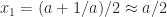
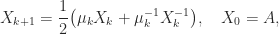
with, for example,

$\notag \mu_k = \sqrt{\|X_k^{-1}\|/\|X_k\|}.$

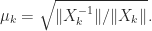
This parameter $\mu_k$ can be computed at no extra cost.

As an example, we took A = gallery('lotkin',4), which has eigenvalues $1.887$ , $-1.980\times10^{-1}$ , $-1.228\times10^{-2}$ , and $-1.441\times10^{-4}$ to four significant figures. After six iterations of the unscaled Newton iteration $X_6$ had an eigenvalue $-100.8$ , showing that $X_6$ is far from $\mathrm{sign}(A)$ , which has eigenvalues $\pm 1$ . Yet when scaled by $\mu_k$ (using the $1$ -norm), after six iterations all the eigenvalues of $X$ were within distance $10^{-16}$ of $\pm 1$ , and the iteration had converged to within this tolerance.

The Matrix Computation Toolbox contains a MATLAB function signm that computes the matrix sign function. It computes a Schur decomposition then obtains the sign of the triangular Schur factor by a finite recurrence. This function is too expensive for use in applications, but is reliable and is useful for experimentation.

Relation to Matrix Square Root and Polar Decomposition

The matrix sign function is closely connected with the matrix square root and the polar decomposition. This can be seen through the relations

$\notag \mathrm{sign}\left( \begin{bmatrix} 0 & A \\\ I & 0 \end{bmatrix} \right ) = \begin{bmatrix}0 & A^{1/2} \\ A^{-1/2} & 0 \end{bmatrix}, \\[\smallskipamount]$

for $A$ with no eigenvalues on the nonpositive real axis, and

$\notag \mathrm{sign}\left( \begin{bmatrix} 0 & A \\\ A^* & 0 \end{bmatrix} \right ) = \begin{bmatrix}0 & U \\ U^* & 0 \end{bmatrix},$

for nonsingular $A$ , where $A = UH$ is a polar decomposition. Among other things, these relations yield iterations for $A^{1/2}$ and $U$ by applying the iterations above to the relevant block $2n\times 2n$ matrix and reading off the (1,2) block.

References

This is a minimal set of references, which contain further useful references within.

Nicholas J. Higham, Functions of Matrices: Theory and Computation, Society for Industrial and Applied Mathematics, Philadelphia, PA, USA, 2008. (Chapter 5.)
Charles Kenney and Alan Laub, Rational Iterative Methods for the Matrix Sign Function, SIAM J. Matrix Anal. Appl. 12(2), 273–291, 1991.
J. D. Roberts, Linear Model Reduction and Solution of the Algebraic Riccati Equation by Use of the Sign Function, Internat. J. Control 32, 677–687, 1980.

What Is the Matrix Sign Function?

Application to Sylvester Equation

Application to the Eigenvalue Problem

Computing the Matrix Sign Function

Relation to Matrix Square Root and Polar Decomposition

References

Related Blog Posts

Leave a Reply Cancel reply

Application to Sylvester Equation

Application to the Eigenvalue Problem

Computing the Matrix Sign Function

Relation to Matrix Square Root and Polar Decomposition

References

Related Blog Posts

Share this:

Related

Leave a Reply Cancel reply