What Is a Symmetric Indefinite Matrix?

A symmetric indefinite matrix $A$ is a symmetric matrix for which the quadratic form $x^TAx$ takes both positive and negative values. By contrast, for a positive definite matrix $x^TAx > 0$ for all nonzero $x$ and for a negative definite matrix $x^TAx < 0$ for all nonzero $x$ .

A neat way to express the indefinitess is that there exist vectors $x$ and $y$ for which $(x^TAx)(y^TAy) < 0$ .

A symmetric indefinite matrix has both positive and negative eigenvalues and in some sense is a typical symmetric matrix. For example, a random symmetric matrix is usually indefinite:

>> rng(3); B = rand(4); A = B + B'; eig(A)'
ans =
  -8.9486e-01  -6.8664e-02   1.1795e+00   3.9197e+00

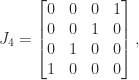
In general it is difficult to tell if a symmetric matrix is indefinite or definite, but there is one easy-to-spot sufficient condition for indefinitess: if the matrix has a zero diagonal element that has a nonzero element in its row then it is indefinite. Indeed if $a_{kk} = 0$ then $e_k^TAe_k = a_{kk} = 0$ , where $e_k$ is the $k$ th unit vector, so $A$ cannot be positive definite or negative definite. The existence of a nonzero element in the row of the zero rules out the matrix being positive semidefinite ( $x^TAx \ge 0$ for all $x$ ) or negative semidefinite ( $x^TAx \le 0$ for all $x$ ).

An example of a symmetric indefinite matrix is a saddle point matrix, which has the block $2\times 2$ form

$\notag C = \begin{bmatrix} A & B^T \\ B & 0 \end{bmatrix},$

where $A$ is symmetric positive definite and $B\ne0$ . When $A$ is the identity matrix, $C$ is the augmented system matrix associated with a least squares problem $\min_x \|Bx - d\|_2$ . Another example is the $n\times n$ reverse identity matrix $J_n$ , illustrated by

$\notag J_4 = \begin{bmatrix} 0 & 0 & 0 & 1 \\ 0 & 0 & 1 & 0 \\ 0 & 1 & 0 & 0 \\ 1 & 0 & 0 & 0 \end{bmatrix},$

which has eigenvalues $\pm1$ (exercise: how many $1$ s and how many $-1$ s?). A third example is a Toeplitz tridiagonal matrix with zero diagonal:

>> A = full(gallery('tridiag',5,1,0,1)), eig(sym(A))'
A =
     0     1     0     0     0
     1     0     1     0     0
     0     1     0     1     0
     0     0     1     0     1
     0     0     0     1     0
ans =
[-1, 0, 1, 3^(1/2), -3^(1/2)]

How can we exploit symmetry in solving a linear system $Ax = b$ with a symmetric indefinite matrix $A$ ? A Cholesky factorization does not exist, but we could try to compute a factorization $A = LDL^T$ , where $L$ is unit lower triangular and $D$ is diagonal with both positive and negative diagonal entries. However, this factorization does not always exist and if it does, its computation in floating-point arithmetic can be numerically unstable. The simplest example of nonexistence is the matrix

$\notag \begin{bmatrix} 0 & 1\\ 1 & 1 \end{bmatrix} \ne \begin{bmatrix} 1 & 0 \\ \ell_{21} & 0 \end{bmatrix} \begin{bmatrix} d_{11} & 0 \\ 0 & d_{22}\end{bmatrix} \begin{bmatrix} 1 & \ell_{21}\\ 0 & 1\end{bmatrix}.$

The way round this is to allow $D$ to have $2 \times 2$ blocks. We can compute a block $\mathrm{LDL^T}$ factorization $PAP^T = LDL^T$ , were $P$ is a permutation matrix, $L$ is unit lower triangular, and $D$ is block diagonal with diagonal blocks of size $1$ or $2$ . Various pivoting strategies, which determine $P$ , are possible, but the recommend one is the symmetric rook pivoting strategy of Ashcraft, Grimes, and Lewis (1998), which has the key property of producing a bounded $L$ factor. Solving $Ax = b$ now reduces to substitutions with $L$ and a solve with $D$ , which involves solving $2\times 2$ linear systems for the $2\times 2$ blocks and doing divisions for the $1\times 1$ blocks (scalars).

MATLAB implements $\mathrm{LDL^T}$ factorization in its ldl function. Here is an example using Anymatrix:

>> A = anymatrix('core/blockhouse',4), [L,D,P] = ldl(A), eigA = eig(A)'
A =
  -4.0000e-01  -8.0000e-01  -2.0000e-01   4.0000e-01
  -8.0000e-01   4.0000e-01  -4.0000e-01  -2.0000e-01
  -2.0000e-01  -4.0000e-01   4.0000e-01  -8.0000e-01
   4.0000e-01  -2.0000e-01  -8.0000e-01  -4.0000e-01
L =
   1.0000e+00            0            0            0
            0   1.0000e+00            0            0
   5.0000e-01  -8.3267e-17   1.0000e+00            0
  -2.2204e-16  -5.0000e-01            0   1.0000e+00
D =
  -4.0000e-01  -8.0000e-01            0            0
  -8.0000e-01   4.0000e-01            0            0
            0            0   5.0000e-01  -1.0000e+00
            0            0  -1.0000e+00  -5.0000e-01
P =
     1     0     0     0
     0     1     0     0
     0     0     1     0
     0     0     0     1
eigA =
  -1.0000e+00  -1.0000e+00   1.0000e+00   1.0000e+00

Notice the $2\times 2$ blocks on the diagonal of $D$ , each of which contains one negative eigenvalue and one positive eigenvalue. The eigenvalues of $D$ are not the same as those of $A$ , but since $A$ and $D$ are congruent they have the same number of positive, zero, and negative eigenvalues.

References

Cleve Ashcraft, Roger Grimes, and John Lewis, Accurate Symmetric Indefinite Linear Equation Solvers, SIAM J. Matrix Anal. Appl. 20, 513–561, 1998.
Nicholas J. Higham and Mantas Mikaitis, Anymatrix: An Extendable MATLAB Matrix Collection, Numer. Algorithms, 90:3, 1175–1196, 2021.

What Is a Symmetric Indefinite Matrix?

References

Related Blog Posts

Leave a comment Cancel reply

References

Related Blog Posts

Share this:

Related

Leave a comment Cancel reply