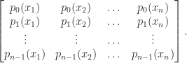
A vector norm measures the size, or length, of a vector. For complex -vectors, a vector norm is a function satisfying
with equality if and only if (nonnegativity),
for all (homogeneity),
for all (the triangle inequality).
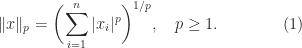
An important class of norms is the Hölder -norms
The -norm is interpreted as and is given by
Other important special cases are
A useful concept is that of the dual norm associated with a given vector norm, which is defined by
The maximum is attained because the definition is equivalent to , in which we are maximizing a continuous function over a compact set. Importantly, the dual of the dual norm is the original norm (Horn and Johnson, 2013, Thm. 5.5.9(c)).
We can rewrite the definition of dual norm, using the homogeneity of vector norms, as
Hence we have the attainable inequality
which is the generalized Hölder inequality.
The dual of the -norm is the -norm, where , so for the -norms the inequality (2) becomes the (standard) Hölder inequality,
An important special case is the Cauchy–Schwarz inequality,
The notation is used to denote the number of nonzero entries in , even though it is not a vector norm and is not obtained from (1) with . In portfolio optimization, if specifies how much to invest in stock then the inequality says “invest in at most stocks”.
In numerical linear algebra, vector norms play a crucial role in the definition of a subordinate matrix norm, as we will explain in the next post in this series.
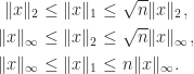
All norms on are equivalent in the sense that for any two norms and there exist positive constants and such that
For example, it is easy to see that
The 2-norm is invariant under unitary transformations: if , then .
Care must be taken to avoid overflow and (damaging) underflow when evaluating a vector -norm in floating-point arithmetic for . One can simply use the formula , but this requires two passes over the data (the first to evaluate ). For more efficient one-pass algorithms for the -norm see Higham (2002, Sec. 21.8) and Harayama et al. (2021).
References
This is a minimal set of references, which contain further useful references within.
The Fugaku supercomputer that tops the HPL-AI mixed-precision benchmark in the June 2021 TOP500 list. It solved a linear system of order 10^7 using IEEE half precision arithmetic for most of the computations.
The largest dense linear systems being solved today are of order , and future exascale computer systems will be able to tackle even larger problems. Rounding error analysis shows that the computed solution satisfies a componentwise backward error bound that, under favorable assumptions, is of order , where is the unit roundoff of the floating-point arithmetic: for double precision and for single precision. This backward error bound cannot guarantee any stability for single precision solution of today’s largest problems and suggests a loss of half the digits in the backward error for double precision.
Half precision floating-point arithmetic is now readily available in hardware, in both the IEEE binary16 format and the bfloat16 format, and it is increasingly being used in machine learning and in scientific computing more generally. For the computation of the inner product of two -vectors the backward error bound is again of order , and this bound exceeds for for both half precision formats, suggesting a potentially complete loss of numerical stability. Yet inner products with are successfully used in half precision computations in practice.
The error bounds I have referred to are upper bounds and so bound the worst-case over all possible rounding errors. Their main purpose is to reveal potential instabilities rather than to provide realistic error estimates. Yet we do need to know the limits of what we can compute, and for mission critical applications we need to be able to guarantee a successful computation..
Can we understand the behavior of linear algebra algorithms at extreme scale and in low precision floating-point arithmetics?
To a large extent the answer is yes if we exploit three different features to obtain smaller error bounds.
Blocked Algorithms
Many algorithms are implemented in blocked form. For example, an inner product of two -vectors and can computed as
where and is the block size. The inner product has been broken into smaller inner products of size , which are computed independently then summed. Many linear algebra algorithms are blocked in an analogous way, where the blocking is into submatrices with rows or columns (or both). Careful analysis of the error analysis shows that a blocked algorithm has an error bound about a factor of smaller than that for the corresponding unblocked algorithm. Practical block sizes for matrix algorithms are typically or , so blocking brings a substantial reduction in the error bounds.
Backward errors for the inner product of two vectors with elements of the form -0.25 + randn, computed in single precision in MATLAB with block size 256.
In fact, one can do even better than an error bound of order . By computing the sum with a more accurate summation method the error constant is further reduced to (this is the FABsum method of Blanchard et al. (2020)).
Architectural Features
Intel x86 processors support an 80-bit extended precision format with a 64-bit significand, which is compatible with that specified in the IEEE standard. When a compiler uses this format with 80-bit registers to accumulate sums and inner products it is effectively working with a unit roundoff of rather than for double precision, giving error bounds smaller by a factor up to .
Some processors have a fused multiply–add (FMA) operation, which computes a combined multiplication and addition with one rounding error instead of two. This results in a reduction in error bounds by a factor .
Mixed precision block FMA operations , with matrices of fixed size, are available on Google tensor processing units, NVIDIA GPUs, and in the ARMv8-A architecture. For half precision inputs these devices can produce results of single precision quality, which can give a significant boost in accuracy when block FMAs are chained together to form a matrix product of arbitrary dimension.
Probabilistic Bounds
Worst-case rounding error bounds suffer from the problem that they are not attainable for most specific sets of data and are unlikely to be nearly attained. Stewart (1990) noted that
To be realistic, we must prune away the unlikely. What is left is necessarily a probabilistic statement.
Theo Mary and I have recently developed probabilistic rounding error analysis, which makes probabilistic assumptions on the rounding errors and derives bounds that hold with a certain probability. The key feature of the bounds is that they are proportional to when a corresponding worst-case bound is proportional to . In the most general form of the analysis (Connolly, Higham, and Mary, 2021), the rounding errors are assumed to be mean independent and of mean zero, where mean independence is a weaker assumption than independence.
Putting the Pieces Together
The different features we have described can be combined to obtain significantly smaller error bounds. If we use a blocked algorithm with block size then in an inner product the standard error bound of order reduces to a probabilistic bound of order , which is a significant reduction. Block FMAs and extended precision registers provide further reductions.
For example, for a linear system of order solved in single precision with a block size of , the probabilistic error bound is of order versus for the standard worst-case bound. If FABsum is used then the bound is further reduced.
Our conclusion is that we can successfully solve linear algebra problems of greater size and at lower precisions than the standard rounding error analysis suggests. A priori bounds will always be pessimistic, though. One should compute a posteriori residuals or backward errors (depending on the problem) in order to assess the quality of a numerical solution.
For full details of the work summarized here, see Higham (2021).
In July 2021, Sven Hammarling, Françoise Tisseur and I organized an online workshop New Directions in Numerical Linear Algebra and High Performance Computing. The workshop brought together researchers working in numerical linear algebra and high performance computing to discuss current developments and challenges in the light of evolving computer hardware. It was held to honour Jack Dongarra on the occasion of his 70th birthday. The workshop had been postponed from July 2020 as a result of the pandemic.
Videos of the talks are now available on the Numerical Linear Algebra Group’s YouTube channel and are included below. Slides for the talks are available on the workshop website.
Sven Hammarling (The University of Manchester), “Jack Dongarra”.
Iain Duff (STFC-RAL and CERFACS), “Jack”
James Demmel (University of California, Berkeley), “New Communication-Avoiding Algorithms, and Fixing Old Bugs in the BLAS and LAPACK”
Piotr Luszczek (University of Tennessee), “Numerical Methods and Across Scales, Precisions and Hardware Platforms”
Cleve Moler (MathWorks), “Computers That I Have Known”
Yves Robert (Ecole Normale Supérieure de Lyon), “25+ Years of Scheduling at ICL”
Françoise Tisseur (The University of Manchester), “Mixed Precision Tall and Thin QR Factorization with Applications”
David Keyes (King Abdullah University of Science and Technology), “Adaptive Nonlinear Preconditioning for PDEs with Error Bounds on Output Functionals”
Zhaojun Bai (University of California, Davis), “Many Eigenpair Computation Via Hotelling’S Deflation”,
Ilse Ipsen (North Carolina State University), “A Few Observations About Summation Algorithms”
Erich Strohmaier (TOP500), “TOP500 and Accidental Benchmarking”
Nick Higham (The University of Manchester), “Solving Dense Linear Systems: A Brief History and Future Directions ”
Jack Dongarra (University of Tennessee, Oak Ridge Laboratory and The University of Manchester), “Still Having Fun After 50 Years”,
The two-part minisymposium Bohemian Matrices and Applications, organized by Rob Corless and I, took place at the SIAM Annual Meeting, July 22 and 23, 2021. This page makes available slides from some of the talks.
The minisymposium followed a two-part minisymposium on Bohemian matrices at the 2019 ICIAM meeting in Valencia and a 3-day workshop on Bohemian matrices in Manchester in 2018.
Minisymposium description: Bohemian matrices are matrices with entries drawn from a fixed discrete set of small integers (or some other discrete set). The term is a contraction of BOunded HEight Matrix of Integers. Such matrices arise in many applications, and include graph incidence matrices and Bernoulli matrices. The questions of interest range from identifying structures in the spectra of particular classes of Bohemian matrix to searching for most ill conditioned matrices within a class, and applications include stress-testing algorithms and software. This minisymposium will report recent theoretical and computational progress as well as open questions.
Putting Skew-Symmetric Tridiagonal Bohemians on the Calendar. Robert M. Corless, Western University, Canada. Abstract. Rob did not use slides but gave his talk using this paper and this Maple worksheet.
Determinants of Normalized Bohemian Upper Hessenberg Matrices. Massimiliano Fasi, Örebro University, Sweden; Jishe Feng, Longdong University, China; Gian Maria Negri Porzio, University of Manchester, United Kingdom. Abstract. Slides.
Experiments on Upper Hessenberg and Toeplitz Bohemians. Eunice Chan, Western University, Canada. Abstract. Slides.
Eigenvalues of Magic Squares and Related Bohemian Matrices. Hariprasad Manjunath Hegde, Indian Institute of Science, Bengaluru, India. Abstract. Slides.
Calculating the 3D Kings Multiplicity Constant. Nicholas Cohen and Neil Calkin, Clemson University, U.S. Abstract. Slides.
Bohemian Inners Inverses: A First Step Toward Bohemian Generalized Inverses. Laureano Gonzalez-Vega, Universidad de Cantabria, Spain; Juan Rafael Sendra, Universidad Alcalá de Henares, Spain; Juana Sendra Pons, Universidad Politécnica de Madrid, Spain. Abstract. Slides.
Recent Progress in the Rational Factorisation of Integer Matrices. Matthew Lettington, Cardiff University, United Kingdom. Abstract. Slides.
Which Columns are Independent? Why does Row Rank = Column Rank? Gilbert Strang, Massachusetts Institute of Technology, U.S. Abstract. Slides.
Bohemian Matrices: the Symbolic Computation Approach. Juana Sendra, Universidad Autónoma de Madrid, Spain; Laureano González-Vega, Universidad de Estudios Financieros en Madrid, Spain; Juan Rafael Sendra, Universidad Alcalá de Henares, Spain. Abstract. Slides.
The determinant of a square submatrix of a matrix is called a minor. A matrix is totally positive if every minor is positive. It is totally nonnegative if every minor is nonnegative. These definitions require, in particular, that all the matrix elements must be nonnegative or positive, as must .
An important property is that total nonnegativity is preserved under matrix multiplication and hence under taking positive integer powers.
Theorem 1.If are totally nonnegative then so is .
Theorem 1 is a direct consequence of the Binet–Cauchy theorem on determinants (also known as the Cauchy–Binet theorem). To state it, we need a way of specifying submatrices. We say the vector is an index vector of order if its components are integers from the set satisfying . If and are index vectors of order and , respectively, then denotes the matrix with () element .
Theorem 2. (Binet–Cauchy) Let , , and . If and are index vectors of order and then
where the sum is over all index vectors of order .
Note than when , (1) reduces to the well-known relation , while when , (1) reduces to the definition of matrix multiplication.
Totally nonnegative matrices have many interesting determinantal properties. For example, they satisfy Fischer’s inequality, first proved for symmetric positive definite matrices.
Theorem 3. (Fischer) If is totally nonnegative then for any index vector ,
where comprises the indices not in .
By repeatedly applying (2) with containing just one element, we obtain Hadamard’s inequality for totally nonnegative :
Examples
We give some examples of totally positive matrices, showing how they can be generated in MATLAB. We use the Anymatrix toolbox.
A matrix well known to be positive definite, but which is also totally positive, is the Hilbert matrix, with . The Hilbert matrix is a particular case of a Cauchy matrix , with for given vectors . A Cauchy matrix is totally positive if and , which follows from the formula
In MATLAB, the Hilbert matrix is hilb(n) and the Cauchy matrix can be generated by gallery('cauchy',x,y) (or anymatrix('gallery/cauchy',x,y)).
The Pascal matrix is totally positive for all (see the section below on bidiagonal factorizations).
The one-parameter correlation matrix with off-diagonal elements given by with , illustrated by
is not totally positive because while the principal minors are all positive, the submatrix has nonpositive determinant. However, the Kac–Murdock–Szegö matrix, with , illustrated by
is totally positive thanks to the decay of the elements way from the diagonal. In MATLAB, the Kac–Murdock–Szegö matrix can be generated by gallery('kms',n,rho).
The lower Hessenberg Toeplitz matrix with all elements on and below the superdiagonal, illustrated for by
is totally nonnegative. It has zero eigenvalues, which appear in a single Jordan block, and its largest eigenvalue is . In MATLAB, this matrix can be generated by anymatrix('core/hessfull01',n). This and other binary totally nonnegative matrices are studied by Brualdi and Kirkland (2010).
Finally, consider a nonnegative bidiagonal matrix factorized into a product of elementary nonnegative bidiagonal matrices (nonnegative means that the elements of the matrix are nonnegative):
It is easy to see by inspection that , , and are totally nonnegative, so is totally nonnegative by Theorem 1. With , we have
which is a product of totally nonnegative matrices and hence is totally nonnegative by Theorem 1. This example clearly generalizes to show that an nonnegative bidiagonal matrix is totally nonnegative.
Inverse
Recall that the inverse of a nonsingular is given by , where
and denotes the submatrix of obtained by deleting row and column . If is nonsingular and totally nonnegative then it follows that has a checkerboard (alternating) sign pattern. Indeed, we can write , where and has nonnegative elements, and in fact it can be shown that is totally nonnegative using Theorem 1, Theorem 6, and (3). For example, here is the inverse of the Pascal matrix:
A totally nonnegative matrix has nonnegative trace and determinant, so the sum and product of its eigenvalues are both nonnegative. In fact, all the eigenvalues are real and nonnegative. Since a Jordan block corresponding to a nonnegative eigenvalue is totally nonnegative any Jordan form with nonnegative eigenvalues is possible. More can be said of is irreducible. Recall that a matrix is irreducible if there does not exist a permutation matrix such that
where and are square, nonempty submatrices.
Theorem 4.If is totally nonnegative then its eigenvalues are all real and nonnegative. If is also irreducible then the positive eigenvalues are distinct.
If is nonsingular and totally nonnegative and irreducible then by the theorem we can write the eigenvalues as . It is known that the eigenvector associated with has sign changes, that is, and ( have opposite signs for values of (any zero elements are deleted before counting sign changes). Note that for , we already know from Perron–Frobenius theory that there is a positive eigenvector . This result is illustrated by the Pascal matrix above:
Note that the number of sign changes (but not the number of negative elements) increases by as we go from one column to the next
The class of nonsingular totally nonnegative irreducible matrices is known as the oscillatory matrices, because such matrices arise in the analysis of small oscillations of elastic systems. An equivalent definition (in fact, the usual definition) is that an oscillatory matrix is a totally nonnegative matrix for which is totally positive for some positive integer .
LU Factorization
The next result shows that a totally nonnegative matrix has an LU factorization with special properties. We will need the following special case of Fischer’s inequality (Theorem 3):
Theorem 5.If is nonsingular and totally nonnegative then it has an LU factorization with and totally nonnegative and the growth factor.
Proof. Since is nonsingular and every minor is nonnegative, (4) shows that for , which guarantees the existence of an LU factorization. That the elements of and are nonnegative follows from explicit determinantal formulas for the elements of and . The total nonnegativity of and is proved by Cryer (1976). Gaussian elimination starts with and computes , since . Thus , . For , ; for , . Thus for all and hence . But , so .
Theorem 5 implies that it is safe to compute the LU factorization without pivoting of a nonsingular totally nonnegativity matrix: the factorization does not break down and it is numerically stable. In fact, the computed LU factors have a strong componentwise form of stability. As shown by De Boor and Pinkus (1977), for small enough unit roundoff the computed factors and will have nonnegative elements and so from the standard backward error result for LU factorization,
we have
which gives and hence
which is about as strong a backward error result as we could hope for. The significance of this result is reduced, however, by the fact that for some important classes of totally nonnegative matrices, including Vandermonde matrices and Cauchy matrices, structure-exploiting linear system solvers exist that are substantially faster, and potentially more accurate, than LU factorization.
Factorization into a Product of Bidiagonal Matrices
We showed above that any nonnegative bidiagonal matrix is totally nonnegative. The next result shows that any nonsingular totally nonnegative matrix has an LU factorization in which and can be factorized into a product of nonnegative bidiagonal matrices.
Theorem 6. (Gasca and Peña, 1996) A nonsingular matrix is totally nonnegative if and only if it it can be factorized as
where is a diagonal matrix with positive diagonal entries and and are unit lower and unit upper bidiagonal matrices, respectively, with the first entries along the subdiagonal of and zero and the rest nonnegative.
An analogue of Theorem 6 holds for totally positive matrices, the only difference being that the last subdiagonal entries of and are positive.
The factorization (5) can be computed by Neville elimination, which is a version of Gaussian elimination in which the eliminations are between adjacent rows, working from the bottom of each column upwards.
This factorization into bidiagonal factors can be used to obtain simple proofs of various properties of totally nonnegative matrices and totally positive matrices (Fallat, 2001). It also provides an efficient way to generates such matrices. If all the parameters in and the and are set to then the Pascal matrix is generated.
Testing for Total Positivity
An matrix has principal minors (ones based on submatrices centred on the diagonal) and minors in total. However, it is not necessary to check all these minors to test for total positivity.
Theorem 7. (Gasca and Peña, 1996) The matrix is totally positive if and only if for all index vectors and such that one of and is and the entries of the other are consecutive integers.
Theorem 7 shows that only minors need to be tested. Gasca and Peña have also show that total nonnegativity can be tested by checking about minors. A more efficient way to test for total nonnegativity is to compute the factorization in Theorem 6 and check the signs of the entries.
Notes
The results we have described show that totally nonnegative and totally positive matrices are analogous in many ways to symmetric positive (semi)definite matrices. The analogies go further because totally nonnegative and totally positive matrices also satisfy eigenvalue interlacing inequalities (albeit weaker than for symmetric matrices) and the eigenvalues of an oscillatory matrix majorize the diagonal elements. See Fallat and Johnson (2011) or Fallat (2014) for details.
References
This is a minimal set of references, which contain further useful references within.
Mariano Gasca and Juan M. Peña, On Factorizations of Totally Positive Matrices, in Mariano Gasca and Charles Micchelli, eds, Total Positivity and Its Applications, 109–130, Springer, 1996.
Shaun M. Fallat, Totally Positive and Totally Nonnegative Matrices, in Handbook of Linear Algebra, Leslie Hogben, ed, 29.1–29.17, Chapman and Hall/CRC, 2014.
Shaun M. Fallat and Charles R. Johnson, Totally Nonnegative Matrices, Princeton University Press, Princeton, NJ, USA, 2011.
A real matrix is nonnegative if all its elements are nonnegative and it is positive if all its elements are positive. Nonnegative matrices arise in a wide variety of applications, for example as matrices of probabilities in Markov processes and as adjacency matrices of graphs. Information about the eigensystem is often essential in these applications.
Perron (1907) proved results about the eigensystem of a positive matrix and Frobenius (1912) extended them to nonnegative matrices.
The following three results of increasing specificity summarize the key spectral properties of nonnegative matrices proved by Perron and Frobenius. Recall that a simple eigenvalue of an matrix is one with algebraic multiplicity , that is, it occurs only once in the set of eigenvalues. We denote by the spectral radius of , the largest absolute value of any eigenvalue of .
Theorem 1. (Perron–Frobenius) If is nonnegative then
is an eigenvalue of ,
there is a nonnegative eigenvector such that .
A matrix is reducible if there is a permutation matrix such that
where and are square, nonempty submatrices; it is irreducible if it is not reducible. Examples of reducible matrices are triangular matrices and matrices with a zero row or column. A positive matrix is trivially irreducible.
Theorem 2. (Perron–Frobenius) If is nonnegative and irreducible then
is an eigenvalue of ,
,
there is a positive eigenvector such that ,
is a simple eigenvalue.
Theorem 3. (Perron) If is positive then Theorem 2 holds and, in addition, for any eigenvalue with .
For nonnegative, irreducible , the eigenvalue is called the Perron root of and the corresponding positive eigenvector , normalized so that , is called the Perron vector.
It is a good exercise to apply the theorems to all binary matrices. Here are some interesting cases.
: Theorem 1 says that is an eigenvalue and and that it has a nonnegative eigenvector. Indeed is an eigenvector. Note that is reducible and is a repeated eigenvalue.
: is irreducible and Theorem 2 says that is a simple eigenvalue with positive eigenvector. Indeed the eigenvalues are and is the Perron vector for the Perron root . This matrix has two eigenvalues of maximal modulus.
: Theorem 3 says that is an eigenvalue with positive eigenvector and that the other eigenvalue has modulus less than . Indeed the eigenvalues are the Perron root , with Perron vector , and .
For another example, consider the irreducible matrix
Note that is a companion matrix and a permutation matrix. Theorem 2 correctly tells us that is an eigenvalue of , and that it has a corresponding positive eigenvector, the Perron vector . Two of the eigenvalues are complex, however, and all three eigenvalues have modulus 1, as they must because is orthogonal.
A stochastic matrix is a nonnegative matrix whose row sums are all equal to . A stochastic matrix satisfies , where , which means that has an eigenvalue , and so . Since for any norm, by taking the -norm we conclude that . For a stochastic matrix, Theorem 1 does not give any further information. If is irreducible then Theorem 2 tells us that is a simple eigenvalue, and if is positive Theorem 3 tells us that every other eigenvalue has modulus less than .
The next result is easily proved using Theorem 3 together with the Jordan canonical form. It shows that the powers of a positive matrix behave like multiples of a rank-1 matrix.
Theorem 4. If is positive, is the Perron vector of , and is the Perron vector of then
Note that in the theorem is a left eigenvector of corresponding to , that is, (since ).
If is stochastic and positive then Theorem 4 is applicable and . If also has unit column sums, so that it is doubly stochastic, then and Theorem 4 says that . We illustrate this result in MATLAB using a scaled magic square matrix.
>> n = 4; M = magic(n), A = M/sum(M(1,:)) % Doubly stochastic matrix.
A =
    16     2     3    13
     5    11    10     8
     9     7     6    12
     4    14    15     1
A =
   4.7059e-01   5.8824e-02   8.8235e-02   3.8235e-01
   1.4706e-01   3.2353e-01   2.9412e-01   2.3529e-01
   2.6471e-01   2.0588e-01   1.7647e-01   3.5294e-01
   1.1765e-01   4.1176e-01   4.4118e-01   2.9412e-02

>> for k = 8:8:32, fprintf('%11.2e',norm(A^k-ones(n)/n,1)), end, disp(' ')
   3.21e-05   7.37e-10   1.71e-14   8.05e-16
References
This is a minimal set of references, which contain further useful references within.
Roger A. Horn and Charles R. Johnson, Matrix Analysis, second edition, Cambridge University Press, 2013. Chapter 8. My review of the second edition.
Carl D. Meyer, Matrix Analysis and Applied Linear Algebra, Society for Industrial and Applied Mathematics, Philadelphia, PA, USA, 2000. Chapter 8.
Helene Shapiro, Linear Algebra and Matrices. Topics for a Second Course, American Mathematical Society, Providence, RI, USA, 2015. Chapter 17.
The Kac–Murdock–Szegö matrix is the symmetric Toeplitz matrix
It was considered by Kac, Murdock, and Szegö (1953), who investigated its spectral properties. It arises in the autoregressive AR(1) model in statistics and signal processing.
The matrix is singular for , as is the rank- matrix , and it is also rank- for , as in this case every column is a multiple of the vector with alternating elements . The determinant . For , is nonsingular and the inverse is the tridiagonal (but not Toeplitz) matrix
For , is positive definite, since every leading principal submatrix has positive determinant, as can also be seen by noting that the inverse is diagonally dominant with positive diagonal, so that is positive definite and hence is positive definite.
For , is positive semidefinite, so it is a correlation matrix for in this range.
For , is totally nonnegative, that is. every submatrix has nonnegative determinant. For , we know that is nonsingular, and it is clearly irreducible, and together with the total nonnegativity these properties imply that the eigenvalues are distinct and positive (this can also be deduced from the fact that the inverse is tridiagonal with nonzero subdiagonal and superdiagonal entries).
It is straightforward to verify that has a factorization with the inverse of a unit lower bidiagonal matrix:
This factorization can be used to prove all the properties stated above.
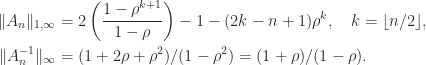
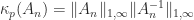
From (1) and (2) we can derive the formulas
Hence we have an explicit formula for the condition number for .
We can allow to be complex, in which case the definition (1) is modified to conjugate the elements below the diagonal. The factorization continues to hold with in replaced by .
The Kac–Murdock–Szegö matrix (for real or complex ) can be generated in MATLAB as gallery('kms',n,rho).
References
This is a minimal set of references, which contain further useful references within.
Ian Gladwell giving talk “Software for the Numerical Solution of ODEs—a University of Manchester and NAG Library Perspective” at Numerical Analysis and Computers—50 Years of Progress, University of Manchester, June 16–17, 1998.
Ian Gladwell passed away on May 23, 2021 at the age of 76. He was born in Bolton, Lancashire in 1944. He did his secondary education at Thornleigh College, Bolton and was an undergraduate at Hertford College, University of Oxford, from where he graduated with a B.A. Hons. in Mathematics in 1966. He did his postgraduate studies at the University of Manchester, gaining an MSc in Numerical Analysis and Computing in 1967 and a PhD in Numerical Analysis in 1970. He was the first PhD student of Christopher T. H. Baker (1939–2017).
Ian was appointed Lecturer in the Department of Mathematics at the University of Manchester in 1969 and progressed to Senior Lecturer in 1980. He was a member of the Numerical Analysis Group (along with Christopher Baker, Len Freeman, George Hall, Will McLewin, Jack Williams (1943–2015), and Joan Walsh (1932–2017)) who, together with colleagues at UMIST, made Manchester a major centre of numerical analysis activity from the 1970s onwards.
Ian’s research focused on ordinary differential equation (ODE) initial value problems and boundary value problems, mathematical software, and parallel computing, and he had a wide knowledge of numerical analysis and scientific computing. He was perhaps best known for his pioneering work on mathematical software for the numerical solution of ODEs, much of which was published in the NAG Library and in the journal ACM Transactions on Mathematical Software. A particular topic of interest for Ian was algorithms and software for the numerical solution of almost block diagonal linear systems, which arise in discretizations of boundary value problems for ODEs and partial differential equations.
More details on Ian’s publications can be found at his MathSciNet author profile (subscription required). It lists 55 publications with 19 co-authors, among which Richard Brankin, Larry Shampine, Ruth Thomas, and Marcin Paprzycki are his most frequent co-authors.
In his time at Manchester he collaborated with a variety of colleagues both inside and outside the department, and he was always ready to offer advice to students and colleagues across the campus on numerical computing (as evidenced by the common sight of people waiting outside his office door to be seen).
Ian was instrumental in setting up the Manchester Numerical Analysis Reports, a long-running technical report series to which he contributed many items.
Ian had a five-month visit to the Department of Computer Science at the University of Toronto in 1975. Links between the Manchester and Toronto departments were strong, and over the years numerical analysts made several visits in both directions.
In the mid 1980s, Ian was one of the first people in the UK to have an email address: igladwel@uk.ac.ucl.cs. His email account was on a computer at University College London (UCL), because UCL hosted a gateway between JANET, the UK computer network, and ARPANET in the USA. Ian kindly allowed Nick Higham and Len Freeman use of the account to communicate with colleagues in the US.
Ian had long-standing collaborations with the Numerical Algorithms Group (NAG) Ltd., Oxford. He contributed many codes and associated documentation to the NAG Library, principally in ordinary differential equations. In a 1979 paper in ACM Trans. Math. Software he wrote
“When the NAG library structure was designed in the late 1960s, it was decided to devote a chapter, named DO2, to the numerical solution of systems of ordinary differential equations and that this chapter would be contributed by members of the Department of Mathematics, University of Manchester, and in particular by J. E. Walsh, G. Hall, and the author.”
Ian was a long-term member of NAG and of the NAG Technical Policy Committee, and during 1986 he held a Royal Society/Science and Engineering Research Council Industrial Fellowship at NAG.
Nick Higham was taught by Ian in an upper level undergraduate course “Numerical Linear Algebra” that Ian was giving for the first time, in 1981. As an MSc student and PhD student he benefited greatly from Ian’s advice about how to think about and do research.
Ian moved to the Department of Mathematics at Southern Methodist University (SMU), Dallas, as a Visiting Associate Professor in 1987, which became a permanent position in 1988. He had collaborated during the 1980s with Larry Shampine, who was working at Sandia National Laboratories until he moved to the SMU Mathematics Department in 1986.
Ian served as chair of the department 1988–1994 and again in 1998. He was also Director of Graduate Studies from 2005–2008. Ian excelled in these roles as mentor, which is recognized by a PhD fellowship in his honor. Jim Nagy was extremely fortunate to have Ian as his first department chair in 1992; Ian mentored him during the challenging tenure-track years, advising on research, teaching and more, including extensive editing of his first successful grant proposals.
Ian wrote the book Solving ODEs with MATLAB (2003) with Larry Shampine and Skip Thompson, which was described as “an excellent treatment of the fundamentals for solving ODEs using MATLAB” in Mathematical Reviews. It is Ian’s most highly cited work, with around 900 citations on Google Scholar at the time of writing.
Ian served as editor for ten journals, including as Associate Editor (2002–2005) and Editor-in-Chief (2005–2008) of ACM Transactions on Mathematical Software, as Associate Editor of the IMA Journal on Numerical Analysis (1988–2007), and as Associate Editor of Scalable Computing: Practice and Experience (2005–2010). A special issue of the latter journal in 2009 was dedicated to him on the occasion of his retirement from SMU
Ian was a long-term member of the Institute of Mathematics and Its Applications, of which he was a Fellow, and the Society for Industrial and Applied Mathematics.
According to the Mathematics Genealogy Project, Ian had 23 PhD students, equally split between Manchester and SMU, with one jointly supervised at the University of Bari.
where the sum is over all permutations ) of the sequence and is the number of inversions in , that is, the number of pairs with . Each term in the sum is a signed product of entries of and the product contains one entry taken from each row and one from each column.
The determinant is sometimes written with vertical bars, as .
Three fundamental properties are
The first property is immediate, the second can be proved using properties of permutations, and the third is proved in texts on linear algebra and matrix theory.
An alternative, recursive expression for the determinant is the Laplace expansion
for any , where denotes the submatrix of obtained by deleting row and column , and for a scalar . This formula is called the expansion by minors because is a minor of .
For some types of matrices the determinant is easy to evaluate. If is triangular then . If is unitary then implies on using (3) and (4). An explicit formula exists for the determinant of a Vandermonde matrix.
The determinant of is connected with the eigenvalues of via the property . Since the eigenvalues are the roots of the characteristic polynomial , this relation follows by setting in the expression
For , the determinant is
but already for the determinant is tedious to write down. If one must compute , the formulas (1) and (5) are too expensive unless is very small: they have an exponential cost. The best approach is to use a factorization of involving factors that are triangular or orthogonal, so that the determinants of the factors are easily computed. If is an LU factorization, with a permutation matrix, unit lower triangular, and upper triangular, then . As this expression indicates, the determinant is prone to overflow and underflow in floating-point arithmetic, so it may be preferable to compute .
The determinant features in the formula
for the inverse, where is the adjugate of (recall that has element ). More generally, Cramer’s rule says that the components of the solution to a linear system are given by , where denotes with its th column replaced by . While mathematically elegant, Cramer’s rule is of no practical use, as it is both expensive and numerically unstable in finite precision arithmetic.
Inequalities
A celebrated bound for the determinant of a Hermitian positive definite matrix is Hadamard’s inequality. Note that for such , is real and positive (being the product of the eigenvalues, which are real and positive) and the diagonal elements are also real and positive (since ).
Theorem 1 (Hadamard’s inequality). For a Hermitian positive definite matrix ,
with equality if and only if is diagonal.
Theorem 1 is easy to prove using a Cholesky factorization.
The following corollary can be obtained by applying Theorem 1 to or by using a QR factorization of .
Corollary 2. For ,
with equality if and only if the columns of are orthogonal.
Obviously, one can apply the corollary to and obtain the analogous bound with column norms replaced by row norms.
The determinant of can be interpreted as the volume of the parallelepiped , whose sides are the columns of . Corollary 2 says that for columns of given lengths the volume is maximized when the columns are orthogonal.
Nearness to Singularity and Conditioning
The determinant characterizes nonsingularity: is singular if and only if . It might be tempting to use as a measure of how close a nonsingular matrix is to being singular, but this measure is flawed, not least because of the sensitivity of the determinant to scaling. Indeed if is unitary then can be given any value by a suitable choice of , yet is perfectly conditioned: , where is the condition number.
To deal with the poor scaling one might normalize the determinant: in view of Corollary 2,
satisfies and if and only if the columns of are orthogonal. Birkhoff (1975) calls the Hadamard condition number. In general, is not related to the condition number , but if has columns of unit -norm then it can be shown that (Higham, 2002, Prob. 14.13). Dixon (1984) shows that for classes of random matrices that include matrices with elements independently drawn from a normal distribution with mean , the probability that the inequality
holds tends to as for any , so for large . This exponential growth is much faster than the growth of , for which Edelman (1998) showed that for the standard normal distribution, , where denotes the mean value. This MATLAB example illustrates these points.
>> rng(1); n = 50; A = randn(n);
>> psi = prod(sqrt(sum(A.*A)))/abs(det(A)), kappa2 = cond(A)
psi =
   5.3632e+10
kappa2 =
   1.5285e+02
>> ratio = psi/(n^(0.25)*exp(n/2))
ratio =
   2.8011e-01
The relative distance from to the set of singular matrices is equal to the reciprocal of the condition number.
Theorem 3 (Gastinel, Kahan). For and any subordinate matrix norm,
Notes
Determinants came before matrices, historically. Most linear algebra textbooks make significant use of determinants, but a lot can be done without them. Axler (1995) shows how the theory of eigenvalues can be developed without using determinants.
Determinants have little application in practical computations, but they are a useful theoretical tool in numerical analysis, particularly for proving nonsingularity.
There is a large number of formulas and identities for determinants. Sir Thomas Muir collected many of them in his five-volume magnum opus The Theory of Determinants in the Historical Order of Development, published between 1890 and 1930. Brualdi and Schneider (1983) give concise derivations of many identities using Gaussian elimination, bringing out connections between the identities.
The quantity obtained by modifying the definition (1) of determinant to remove the term is the permanent. The permanent arises in combinatorics and quantum mechanics and is much harder to compute than the determinant: no algorithm is known for computing the permanent in operations for a polynomial .
References
This is a minimal set of references, which contain further useful references within.
Sheldon Axler, Down With Determinants!, Amer. Math. Monthly 102, 139–154, 1995.
A Vandermonde matrix is defined in terms of scalars , , …, by
The are called points or nodes. Note that while we have indexed the nodes from , they are usually indexed from in papers concerned with algorithms for solving Vandermonde systems.
Vandermonde matrices arise in polynomial interpolation. Suppose we wish to find a polynomial of degree at most that interpolates to the data , that is, , . These equations are equivalent to
where is the vector of coefficients. This is known as the dual problem. We know from polynomial interpolation theory that there is a unique interpolant if the are distinct, so this is the condition for to be nonsingular.
The problem
is called the primal problem, and it arises when we determine the weights for a quadrature rule: given moments find weights such that , .
Determinant
The determinant of is a function of the points . If for some then has identical th and th columns, so is singular. Hence the determinant must have a factor . Consequently, we have
where, since both sides have degree in the , is a constant. But contains a term (from the main diagonal), so . Hence
This formula confirms that is nonsingular precisely when the are distinct.
Inverse
Now assume that is nonsingular and let . Equating elements in the th row of gives
where is the Kronecker delta (equal to if and otherwise). These equations say that the polynomial takes the value at and at , . It is not hard to see that this polynomial is the Lagrange basis polynomial:
We deduce that
where denotes the sum of all distinct products of of the arguments (that is, is the th elementary symmetric function).
From (1) and (3) we see that if the are real and positive and arranged in increasing order and has a checkerboard sign pattern: the element has sign .
Note that summing (2) over gives
where the second equality follows from the fact that is a degree polynomial that takes the value at the distinct points . Hence
so the elements in the th column of the inverse sum to for and for .
Example
To illustrate the formulas above, here is an example, with and :
for which .
Conditioning
Vandermonde matrices are notorious for being ill conditioned. The ill conditioning stems from the monomials being a poor basis for the polynomials on the real line. For arbitrary distinct points , Gautschi showed that satisfies
with equality on the right when for all with a fixed (in particular, when for all ). Note that the upper and lower bounds differ by at most a factor . It is also known that for any set of real points ,
and that for we have , where the lower bound is an extremely fast growing function of the dimension!
These exponential lower bounds are alarming, but they do not necessarily rule out the use of Vandermonde matrices in practice. One of the reasons is that there are specialized algorithms for solving Vandermonde systems whose accuracy is not dependent on the condition number , and which in some cases can be proved to be highly accurate. The first such algorithm is an operation algorithm for solving of Björck and Pereyra (1970). There is now a long list of generalizations of this algorithm in various directions, including for confluent Vandermonde-like matrices (Higham, 1990), as well as for more specialized problems (Demmel and Koev, 2005) and more general ones (Bella et al., 2009). Another important observation is that the exponential lower bounds are for real nodes. For complex nodes can be much better conditioned. Indeed when the are the roots of unity, is the unitary Fourier matrix and so is perfectly conditioned.
Generalizations
Two ways in which Vandermonde matrices have been generalized are by allowing confluency of the points and by replacing the monomials by other polynomials. Confluency arises when the are not distinct. If we assume that equal are contiguous then a confluent Vandermonde matrix is obtained by “differentiating” the previous column for each of the repeated points. For example, with points we obtain
The transpose of a confluent Vandermonde matrix arises in Hermite interpolation; it is nonsingular if the points corresponding to the “nonconfluent columns” are distinct (that is, if in the case of (4)).
A Vandermonde-like matrix is defined in terms of a set of polynomials with having degree :
Of most interest are polynomials that satisfy a three-term recurrence, in particular, orthogonal polynomials. Such matrices can be much better conditioned than general Vandermonde matrices.
Notes
Algorithms for solving confluent Vandermonde-like systems and their rounding error analysis are described in the chapter “Vandermonde systems” of Higham (2002).
Gautschi has written many papers on the conditioning of Vandermonde matrices, beginning in 1962. We mention just his most recent paper on this topic: Gautschi (2011).
References
This is a minimal set of references, which contain further useful references within.


with equality if and only if
(nonnegativity),
for all
(homogeneity),
for all
(the triangle inequality).


 , and future exascale computer systems will be able to tackle even larger problems. Rounding error analysis shows that the computed solution satisfies a componentwise backward error bound that, under favorable assumptions, is of order
  , where
  is the unit roundoff of the floating-point arithmetic:
  for double precision and
  for single precision. This backward error bound cannot guarantee any stability for single precision solution of today’s largest problems and suggests a loss of half the digits in the backward error for double precision.
 for
for  for both half precision formats, suggesting a potentially complete loss of numerical stability. Yet inner products with
  of two
  can computed as
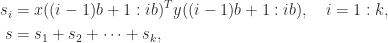
 and
and  is the block size. The inner product has been broken into
  , which are computed independently then summed. Many linear algebra algorithms are blocked in an analogous way, where the blocking is into submatrices with
  or
or  , so blocking brings a substantial reduction in the error bounds.
 . By computing the sum
  with a more accurate summation method the error constant is further reduced to
  (this is the FABsum method of Blanchard et al. (2020)).
 rather than
  for double precision, giving error bounds smaller by a factor up to
  .
. with one rounding error instead of two. This results in a reduction in error bounds by a factor
  , with matrices
  of fixed size, are available on Google tensor processing units, NVIDIA GPUs, and in the ARMv8-A architecture. For half precision inputs these devices can produce results of single precision quality, which can give a significant boost in accuracy when block FMAs are chained together to form a matrix product of arbitrary dimension.
 when a corresponding worst-case bound is proportional to
  , which is a significant reduction. Block FMAs and extended precision registers provide further reductions.
 solved in single precision with a block size of
  versus
 graph incidence matrices and
  Bernoulli matrices. The questions of interest range from identifying structures in the spectra of particular classes of Bohemian matrix to searching for most ill conditioned matrices within a class, and applications include stress-testing algorithms and software. This minisymposium will report recent theoretical and computational progress as well as open questions.
 is totally positive if every minor is positive. It is totally nonnegative if every minor is nonnegative. These definitions require, in particular, that all the matrix elements must be nonnegative or positive, as must
  .
. are totally nonnegative then so is
  .
.![\alpha = [\alpha_1,\alpha_2,\dots,\alpha_k]](https://s0.wp.com/latex.php?latex=%5Calpha+%3D+%5B%5Calpha_1%2C%5Calpha_2%2C%5Cdots%2C%5Calpha_k%5D&bg=ffffff&fg=222222&s=0&c=20201002) is an index vector of order
is an index vector of order  satisfying
  . If
. If  and
and  are index vectors of order
  , respectively, then
  denotes the
  matrix with (
 ) element
  .
. ,
,  , and
, and  . If
. If  then
then
 of order
  , (1) reduces to the well-known relation
  , while when
  , (1) reduces to the definition of matrix multiplication.
 comprises the indices not in
  :
:
 , with
  . The Hilbert matrix is a particular case of a Cauchy matrix
  , with
  for given vectors
  . A Cauchy matrix is totally positive if
  and
and  , which follows from the formula

 satisfy
 is defined by
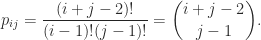
 with off-diagonal elements given by
  with
with  , illustrated by
![A([1,2],[2,3]) = \bigl[\begin{smallmatrix} \theta & \theta \\ 1 & \theta \end{smallmatrix}\bigr]](https://s0.wp.com/latex.php?latex=A%28%5B1%2C2%5D%2C%5B2%2C3%5D%29+%3D++++%5Cbigl%5B%5Cbegin%7Bsmallmatrix%7D++++%5Ctheta+%26+%5Ctheta+%5C%5C++++1++++++%26+%5Ctheta++++%5Cend%7Bsmallmatrix%7D%5Cbigr%5D+&bg=ffffff&fg=222222&s=0&c=20201002) has nonpositive determinant. However, the
has nonpositive determinant. However, the  , with
 with all elements
  by
by
 zero eigenvalues, which appear in a single Jordan block, and its largest eigenvalue is
  . In MATLAB, this matrix can be generated by
  bidiagonal matrix factorized into a product of elementary nonnegative bidiagonal matrices (nonnegative means that the elements of the matrix are nonnegative):
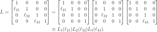
 ,
,  , and
, and  are totally nonnegative, so
  is totally nonnegative by Theorem 1. With
  , we have
 nonnegative bidiagonal matrix is totally nonnegative.
 , where
 denotes the submatrix of
  has a checkerboard (alternating) sign pattern. Indeed, we can write
  , where
  and
and  has nonnegative elements, and in fact it can be shown that
  is irreducible if there does not exist a permutation matrix
  such that
 and
and  are square, nonempty submatrices.
 . It is known that the eigenvector
  has
has  sign changes, that is,
  and (
and ( have opposite signs for
  (any zero elements are deleted before counting sign changes). Note that for
  , we already know from Perron–Frobenius theory that there is a positive eigenvector
  . This result is illustrated by the Pascal matrix above:
 is totally positive for some positive integer
 totally nonnegative and the
  .
. for
for  , which guarantees the existence of an LU factorization. That the elements of
  and computes
  , since
  . Thus
  ,
,  . For
. For  ,
,  ; for
; for  ,
,  . Thus
  for all
  and hence
  . But
. But  , so
, so  .
. and
and  will have nonnegative elements and so from the standard backward error result for LU factorization,

 and hence

 is a diagonal matrix with positive diagonal entries and
  and
and  are unit lower and unit upper bidiagonal matrices, respectively, with the first
  entries along the subdiagonal of
  zero and the rest nonnegative.
 subdiagonal entries of
  principal minors (ones based on submatrices centred on the diagonal) and
  minors in total. However, it is not necessary to check all these minors to test for total positivity.
 for all index vectors
 ![[1,2,\dots,k]](https://s0.wp.com/latex.php?latex=%5B1%2C2%2C%5Cdots%2Ck%5D&bg=ffffff&fg=222222&s=0&c=20201002) and the entries of the other are
and the entries of the other are  minors need to be tested. Gasca and Peña have also show that total nonnegativity can be tested by checking about
  minors. A more efficient way to test for total nonnegativity is to compute the factorization in Theorem 6 and check the signs of the entries.
 the spectral radius of
  .
. ,
, ,
, for any eigenvalue
  with
with  .
. , is called the Perron vector.
 matrices. Here are some interesting cases.
![A = \bigl[\begin{smallmatrix}0 & 1 \\ 0 & 0 \end{smallmatrix}\bigr]](https://s0.wp.com/latex.php?latex=A+%3D+%5Cbigl%5B%5Cbegin%7Bsmallmatrix%7D0+%26+1+%5C%5C+0+%26+0+%5Cend%7Bsmallmatrix%7D%5Cbigr%5D&bg=ffffff&fg=222222&s=0&c=20201002) : Theorem 1 says that
: Theorem 1 says that  is an eigenvalue and and that it has a nonnegative eigenvector. Indeed
 ![[1~0]^T](https://s0.wp.com/latex.php?latex=%5B1%7E0%5D%5ET&bg=ffffff&fg=222222&s=0&c=20201002) is an eigenvector. Note that
is an eigenvector. Note that  is a repeated eigenvalue.
![A = \bigl[\begin{smallmatrix}0 & 1 \\ 1 & 0 \end{smallmatrix}\bigr]](https://s0.wp.com/latex.php?latex=A+%3D+%5Cbigl%5B%5Cbegin%7Bsmallmatrix%7D0+%26+1+%5C%5C+1+%26+0+%5Cend%7Bsmallmatrix%7D%5Cbigr%5D&bg=ffffff&fg=222222&s=0&c=20201002) :
:  and
and ![[1~1]^T/2](https://s0.wp.com/latex.php?latex=%5B1%7E1%5D%5ET%2F2&bg=ffffff&fg=222222&s=0&c=20201002) is the Perron vector for the Perron root
is the Perron vector for the Perron root ![A = \bigl[\begin{smallmatrix}1 & 1 \\ 1 & 1 \end{smallmatrix}\bigr]](https://s0.wp.com/latex.php?latex=A+%3D+%5Cbigl%5B%5Cbegin%7Bsmallmatrix%7D1+%26+1+%5C%5C+1+%26+1+%5Cend%7Bsmallmatrix%7D%5Cbigr%5D&bg=ffffff&fg=222222&s=0&c=20201002) : Theorem 3 says that
: Theorem 3 says that  is an eigenvalue with positive eigenvector and that the other eigenvalue has modulus less than
 is an eigenvalue of
 ![[1~1~1]^T/3](https://s0.wp.com/latex.php?latex=%5B1%7E1%7E1%5D%5ET%2F3&bg=ffffff&fg=222222&s=0&c=20201002) . Two of the eigenvalues are complex, however, and all three eigenvalues have modulus 1, as they must because
. Two of the eigenvalues are complex, however, and all three eigenvalues have modulus 1, as they must because  , where
 ![e = [1,1,\dots,1]^T](https://s0.wp.com/latex.php?latex=e+%3D+%5B1%2C1%2C%5Cdots%2C1%5D%5ET&bg=ffffff&fg=222222&s=0&c=20201002) , which means that
, which means that  . Since
  for any norm, by taking the
  then
then
 (since
  ).
). . If
. If  and Theorem 4 says that
  . We illustrate this result in MATLAB using a scaled magic square matrix.
 , as
, as  is the rank-
 , and it is also rank-
 , as in this case every column is a multiple of the vector with alternating elements
 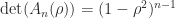 . For
. For  ,
,  is nonsingular and the inverse is the tridiagonal (but not Toeplitz) matrix
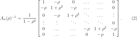
 ,
,  is positive definite, since every leading principal submatrix has positive determinant, as can also be seen by noting that the inverse is diagonally dominant with positive diagonal, so that
  is positive definite and hence
  ,
,  in this range.
 ,
,  , we know that
  with
with 
 for
for  .
. continues to hold with
  replaced by
  .
.

 permutations
  ) of the sequence
  and
and  is the number of inversions in
  , that is, the number of pairs
  with
with  . Each term in the sum is a signed product of
  .
.

 , where
  denotes the
  submatrix of
  for a scalar
  . This formula is called the expansion by minors because
  is a minor of
  is triangular then
  . If
. If  is unitary then
  on using (3) and (4). An
  of
of  . Since the eigenvalues are the roots of the characteristic polynomial
  , this relation follows by setting
  in the expression
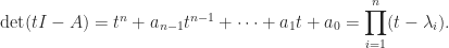
 , the determinant is
 the determinant is tedious to write down. If one must compute
  is an LU factorization, with
  . As this expression indicates, the determinant is prone to overflow and underflow in floating-point arithmetic, so it may be preferable to compute
  .
.
 is the
  element
  ). More generally, Cramer’s rule says that the components of the solution to a linear system
  are given by
  , where
  denotes
  is Hadamard’s inequality. Note that for such
  ,
,  is real and positive (being the product of the eigenvalues, which are real and positive) and the diagonal elements are also real and positive (since
  ).
).
 or by using a QR factorization of
 ![A = [a_1,a_2,\dots,a_n] \in\mathbb{C}^{n\times n}](https://s0.wp.com/latex.php?latex=A+%3D+%5Ba_1%2Ca_2%2C%5Cdots%2Ca_n%5D+%5Cin%5Cmathbb%7BC%7D%5E%7Bn%5Ctimes+n%7D&bg=ffffff&fg=222222&s=0&c=20201002) ,
,
 and obtain the analogous bound with column norms replaced by row norms.
 , whose sides are the columns of
  . It might be tempting to use
  as a measure of how close a nonsingular matrix
  can be given any value by a suitable choice of
  is perfectly conditioned:
  , where
  is the condition number.
 and
and  if and only if the columns of
  the Hadamard condition number. In general,
  , but if
  (Higham, 2002, Prob. 14.13). Dixon (1984) shows that for classes of
 for any
  , so
, so  for large
  , where
  denotes the mean value. This MATLAB example illustrates these points.
 term is the permanent. The permanent arises in combinatorics and quantum mechanics and is much harder to compute than the determinant: no algorithm is known for computing the permanent in
  operations for a polynomial
  , …,
, …,  by
by
 of degree at most
  that interpolates to the data
  , that is,
  ,
,  . These equations are equivalent to
![a = [a_1,a_2,\dots,a_n]^T](https://s0.wp.com/latex.php?latex=a+%3D+%5Ba_1%2Ca_2%2C%5Cdots%2Ca_n%5D%5ET&bg=ffffff&fg=222222&s=0&c=20201002) is the vector of coefficients. This is known as the dual problem. We know from polynomial interpolation theory that there is a unique interpolant if the
is the vector of coefficients. This is known as the dual problem. We know from polynomial interpolation theory that there is a unique interpolant if the  to be nonsingular.
 find weights
  such that
  ,
,  for some
  then
then  . Consequently, we have
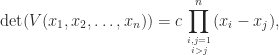
 in the
  is a constant. But
  contains a term
  (from the main diagonal), so
  . Hence
 . Equating elements in the
  gives
gives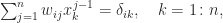
 is the Kronecker delta (equal to
  and
and  takes the value
  and
and  ,
,  . It is not hard to see that this polynomial is the Lagrange basis polynomial:
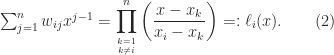

 denotes the sum of all distinct products of
  (that is,
  is the
  and
and  has a checkerboard sign pattern: the
  .
.
 is a degree
 and
and  .
. and
and  :
:![\notag V = \left[\begin{array}{ccccc} 1 & 1 & 1 & 1 & 1\\ 0 & \frac{1}{4} & \frac{1}{2} & \frac{3}{4} & 1\\[\smallskipamount] 0 & \frac{1}{16} & \frac{1}{4} & \frac{9}{16} & 1\\[\smallskipamount] 0 & \frac{1}{64} & \frac{1}{8} & \frac{27}{64} & 1\\[\smallskipamount] 0 & \frac{1}{256} & \frac{1}{16} & \frac{81}{256} & 1 \end{array}\right], \quad V^{-1} = \left[\begin{array}{ccccc} 1 & -\frac{25}{3} & \frac{70}{3} & -\frac{80}{3} & \frac{32}{3}\\[\smallskipamount] 0 & 16 & -\frac{208}{3} & 96 & -\frac{128}{3}\\ 0 & -12 & 76 & -128 & 64\\[\smallskipamount] 0 & \frac{16}{3} & -\frac{112}{3} & \frac{224}{3} & -\frac{128}{3}\\[\smallskipamount] 0 & -1 & \frac{22}{3} & -16 & \frac{32}{3} \end{array}\right],](https://s0.wp.com/latex.php?latex=%5Cnotag+V+%3D+%5Cleft%5B%5Cbegin%7Barray%7D%7Bccccc%7D+1+%26+1+%26+1+%26+1+%26+1%5C%5C+0+%26+%5Cfrac%7B1%7D%7B4%7D+%26+%5Cfrac%7B1%7D%7B2%7D+%26+%5Cfrac%7B3%7D%7B4%7D+%26+1%5C%5C%5B%5Csmallskipamount%5D+0+%26+%5Cfrac%7B1%7D%7B16%7D+%26+%5Cfrac%7B1%7D%7B4%7D+%26+%5Cfrac%7B9%7D%7B16%7D+%26+1%5C%5C%5B%5Csmallskipamount%5D+0+%26+%5Cfrac%7B1%7D%7B64%7D+%26+%5Cfrac%7B1%7D%7B8%7D+%26+%5Cfrac%7B27%7D%7B64%7D+%26+1%5C%5C%5B%5Csmallskipamount%5D+0+%26+%5Cfrac%7B1%7D%7B256%7D+%26+%5Cfrac%7B1%7D%7B16%7D+%26+%5Cfrac%7B81%7D%7B256%7D+%26+1+%5Cend%7Barray%7D%5Cright%5D%2C+%5Cquad+V%5E%7B-1%7D+%3D+%5Cleft%5B%5Cbegin%7Barray%7D%7Bccccc%7D+1+%26+-%5Cfrac%7B25%7D%7B3%7D+%26+%5Cfrac%7B70%7D%7B3%7D+%26+-%5Cfrac%7B80%7D%7B3%7D+%26+%5Cfrac%7B32%7D%7B3%7D%5C%5C%5B%5Csmallskipamount%5D+0+%26+16+%26+-%5Cfrac%7B208%7D%7B3%7D+%26+96+%26+-%5Cfrac%7B128%7D%7B3%7D%5C%5C+0+%26+-12+%26+76+%26+-128+%26+64%5C%5C%5B%5Csmallskipamount%5D+0+%26+%5Cfrac%7B16%7D%7B3%7D+%26+-%5Cfrac%7B112%7D%7B3%7D+%26+%5Cfrac%7B224%7D%7B3%7D+%26+-%5Cfrac%7B128%7D%7B3%7D%5C%5C%5B%5Csmallskipamount%5D+0+%26+-1+%26+%5Cfrac%7B22%7D%7B3%7D+%26+-16+%26+%5Cfrac%7B32%7D%7B3%7D+%5Cend%7Barray%7D%5Cright%5D%2C+&bg=ffffff&fg=222222&s=0&c=20201002)
 .
. satisfies
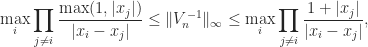
 for all
  for all
  . It is also known that for any set of real points
 we have
  , where the lower bound is an extremely fast growing function of the dimension!
 operation algorithm for solving
  of Björck and Pereyra (1970). There is now a long list of generalizations of this algorithm in various directions, including for confluent Vandermonde-like matrices (Higham, 1990), as well as for more specialized problems (Demmel and Koev, 2005) and more general ones (Bella et al., 2009). Another important observation is that the exponential lower bounds are for real nodes. For complex nodes
  can be much better conditioned. Indeed when the
  is the unitary Fourier matrix and so
  we obtain
 in the case of (4)).
 with
with  having degree