Singular Value Inequalities

Recall that the singular value decomposition (SVD) of a matrix $A \in\mathbb{C}^{m\times n}$ is a factorization $A = U\Sigma V^*$ , where $U\in\mathbb{C}^{m\times m}$ and $V\in\mathbb{C}^{n\times n}$ are unitary and $\Sigma = \mathrm{diag}(\sigma_1,\dots, \sigma_p)\in\mathbb{R}^{m\times n}$ , with $\sigma_1\ge \sigma_2\ge \cdots \ge \sigma_p \ge 0$ , where where $p = \min(m,n)$ . We sometimes write $\sigma_i(A)$ to specify the matrix to which the singular value belongs.

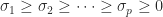
A standard technique for obtaining singular value inequalities for $A$ is to apply eigenvalue inequalities to the Hermitian positive semidefinite matrices $A^*A$ or $AA^*$ , whose eigenvalues are the squares of the singular values of $A$ , or to the Hermitian matrix

$\notag \begin{bmatrix} 0 & A \\ A^* & 0 \end{bmatrix}, \qquad (1)$

whose eigenvalues are plus and minus the singular values of $A$ together with $|m-n|$ zero eigenvalues if $m\ne n$ .

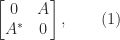
We begin with a variational characterization of singular values.

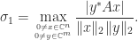
Theorem 1. For $A\in\mathbb{C}^{m\times n}$ ,

$\notag \begin{aligned} \sigma_k &= \min_{\dim(S)=n-k+1} \, \max_{0\ne x\in S} \frac{\|Ax\|_2}{\|x\|_2}\\ &= \max_{\dim(S)= k} \, \min_{0\ne x\in S} \frac{\|Ax\|_2}{\|x\|_2}, \quad k=1\colon \min(m,n), \end{aligned}$

where $S\subseteq \mathbb{C}^n$ .

Proof. The result is obtained by applying the Courant–Fischer theorem (a variational characterization of eigenvalues) to $A^*A$ . $~\square$

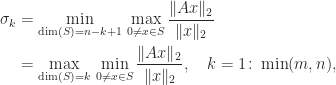
As a special case of Theorem 1, we have

$\notag \sigma_1 = \displaystyle\max_{x \ne 0}\frac{ \|Ax\|_2 }{ \|x\|_2 }, \qquad (2)$

and, for $m\ge n$ ,

$\notag \sigma_n = \displaystyle\min_{x \ne 0}\frac{ \|Ax\|_2 }{ \|x\|_2 }. \qquad (3)$

The expression in the theorem can be rewritten using 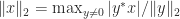$\|x\|_2 = \max_{y\ne 0}|y^*x|/\|y\|_2$ (the equality case in the Cauchy–Schwarz inequality). For example, (2) is equivalent to

$\notag \sigma_1 = \displaystyle\max_{0\ne x\in \mathbb{C}^n\atop 0 \ne y \in \mathbb{C}^m} \displaystyle\frac{|y^*Ax|}{\|x\|_2\|y\|_2}.$

Our first perturbation result bounds the change in a singular value.

Theorem 2. For $A,B\in\mathbb{C}^{m\times n}$ ,

$\notag |\sigma_i(A) - \sigma_i(B)| \le \|A - B \|_2, \quad i = 1\colon \min(m,n). \qquad (4)$

Proof. The bound is obtained by applying the corresponding result for the Hermitian eigenvalue problem to (1). $~\square$

The bound (4) says that the singular values of a matrix are well conditioned under additive perturbation. Now we consider multiplicative perturbations.

The next result is an analogue for singular values of Ostrowski’s theorem for eigenvalues.

Theorem 3. For $A\in \mathbb{C}^{m\times n}$ and nonsingular $X\in\mathbb{C}^{n\times n}$ and $Y\in\mathbb{C}^{m\times m}$ ,

$\notag \sigma_i(Y^*AX) = \theta_i \sigma_i(A), \quad i = 1\colon \min(m,n), \qquad (5)$

where $\sigma_n(X)\sigma_m(Y) \le \theta_i \le \sigma_1(X) \sigma_1(Y)$ .

A corollary of this result is

$\notag |\sigma_i(A) - \sigma_i(Y^*AX)| \le \sigma_i(A) \epsilon, \quad i = 1\colon \min(m,n), \qquad (6)$

where $\epsilon = \max(\|X^*X - I\|_2,\|Y^*Y - I\|_2)$ . The bounds (5) and (6) are intuitively reasonable, because unitary transformations preserve singular values and the bounds quantify in different ways how close $X$ and $Y$ are to being unitary.

Next, we have an interlacing property.

Theorem 4. Let $A\in\mathbb{C}^{m\times n}$ , $A_k = A(:,1\colon k)$ , and $q = \min(m,k)$ . Then

$\notag \sigma_{i+1}(A_{k+1}) \le \sigma_i(A_k) \le \sigma_i(A_{k+1}), \quad i=1\colon q, \quad k = 1\colon n-1,$

where we define $\sigma_{q+1}(A_{k+1}) = 0$ if $m < k+1$ .

Proof. The result is obtained by applying the Cauchy interlace theorem to $A^*A$ , noting that $A_k^*A_k$ is the leading principal submatrix of order $k$ of $A^*A$ . $~\square$

An analogous result holds with rows playing the role of columns (just apply Theorem 4 to $A^*$ ).

Theorem 4 encompasses two different cases, which we illustrate with $i = q$ and $k = n-1$ . The first case is $m \ge n$ , so that $q = n-1$ and

$\notag \sigma_n(A) \le \sigma_{n-1}(A_{n-1}) \le \sigma_{n-1}(A).$

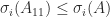
The second case is $m < n$ , so $q = m$ and

$\notag 0 \le \sigma_m(A_{n-1}) \le \sigma_m(A).$

Therefore Theorem 3 shows that removing a column from $A$ does not increase any singular value and that when $m\ge n$ no singular value decreases below $\sigma_n(A)$ . However, when $m < n$ the smallest singular value of $A_{n-1}$ may be less than the smallest singular value of $A$ .

Here is a numerical example. Note that transposing $A$ does not change its singular values.

>> rng(1), A = rand(5,4); % Case 1.
>> B = A(:,1:end-1); sv_A = svd(A)', sv_B = svd(B)'
sv_A =
   1.7450e+00   6.4492e-01   5.5015e-01   3.2587e-01
sv_B =
   1.5500e+00   5.8472e-01   3.6128e-01
> A = A'; B = A(:,1:end-1); sv_B = svd(B)' % Case 2
sv_B =
   1.7098e+00   6.0996e-01   4.6017e-01   1.0369e-01

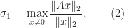
By applying Theorem 4 repeatedly we find that if we partition $A = [A_{11}~A_{12}]$ then $\sigma_i(A_{11}) \le \sigma_i(A)$ for all $i$ for which the left-hand side is defined.

References

Roger A. Horn and Charles R. Johnson, Matrix Analysis, second edition, Cambridge University Press, 2013. My review of the second edition.
Ilse Ipsen, Relative Perturbation Results for Matrix Eigenvalues and Singular Values, Acta Numerica 7, 151–201, 1998.

Singular Value Inequalities

References

Related Blog Posts

3 thoughts on “Singular Value Inequalities”

Leave a Reply Cancel reply

References

Related Blog Posts

Share this:

Related

3 thoughts on “Singular Value Inequalities”

Leave a Reply Cancel reply