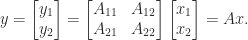
In many applications a matrix 


What is usually wanted is a factorization that displays how close

where 
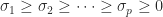


and that the minimum is attained at

so 


Although the SVD is expensive to compute, it may not be significantly more expensive than alternative factorizations. However, the SVD is expensive to update when a row or column is added to or removed from the matrix, as happens repeatedly in signal processing applications.
Many different definitions of a rank-revealing factorization have been given, and they usually depend on a particular matrix factorization. We will use the following general definition.
Definition 1. A rank-revealing factorization (RRF) of

where
,
is diagonal and nonsingular, and
and
are well conditioned.
An RRF concentrates the rank deficiency and ill condition of

where 
Without loss of generality we can assume that

(since 


so 


Definition 2 is a strong requirement, since it requires all the singular values of
Numerical Rank
An RRF helps to determine the numerical rank, which we now define.
Definition 2. For a given
the numerical rank of
.
By the Eckart–Young theorem, the numerical rank is the smallest rank attained over all 


QR Factorization
One might attempt to compute an RRF by using a QR factorization 


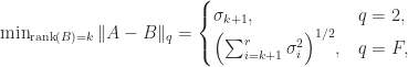
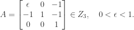
However, it is easy to see that QR factorization in its basic form is flawed as a means for computing an RRF. Consider the matrix
which is a Jordan block with zero eigenvalue. This matrix is its own QR factorization (


![[a_1,a_2,a_3,a_4]](https://s0.wp.com/latex.php?latex=%5Ba_1%2Ca_2%2Ca_3%2Ca_4%5D&bg=ffffff&fg=222222&s=0&c=20201002)
![[a_2,a_3,a_4,a_1]](https://s0.wp.com/latex.php?latex=%5Ba_2%2Ca_3%2Ca_4%2Ca_1%5D&bg=ffffff&fg=222222&s=0&c=20201002)

For a less trivial example, consider the matrix
![\notag A = \left[\begin{array}{rrrr} 1 & 1 &\theta &0\\ 1 & -1 & 2 &1 \\ 1 & 0 &1+\theta &-1\\ 1 &-1 & 2 &-1 \end{array}\right], \quad \theta = 10^{-8}. \qquad (\dagger)](https://s0.wp.com/latex.php?latex=%5Cnotag+++A+%3D+%5Cleft%5B%5Cbegin%7Barray%7D%7Brrrr%7D++++++++1+%26+1++%26%5Ctheta+%260%5C%5C++++++++1+%26+-1+%26+2+%261+%5C%5C++++++++1+%26+0++%261%2B%5Ctheta+%26-1%5C%5C++++++++1+%26-1++%26+2+%26-1+++%5Cend%7Barray%7D%5Cright%5D%2C+%5Cquad+%5Ctheta+%3D+10%5E%7B-8%7D.+%5Cqquad+%28%5Cdagger%29+&bg=ffffff&fg=222222&s=0&c=20201002)
Computing the QR factorization we obtain
R =
  -2.0000e+00   5.0000e-01  -2.5000e+00   5.0000e-01
            0   1.6583e+00  -1.6583e+00  -1.5076e-01
            0            0  -4.2640e-09   8.5280e-01
            0            0            0  -1.4142e+00
The 


QR Factorization With Column Pivoting
A common method for computing an RRF is QR factorization with column pivoting, which for a matrix 

In particular,

If 
![\notag R = \begin{array}[b]{@{\mskip33mu}c@{\mskip-16mu}c@{\mskip-10mu}c@{}} \scriptstyle k & \scriptstyle n-k & \\ \multicolumn{2}{c}{ \left[\begin{array}{c@{~}c@{~}} R_{11}& R_{12} \\ 0 & R_{22} \\ \end{array}\right]} & \mskip-12mu\ \begin{array}{c} \scriptstyle k \\ \scriptstyle n-k \end{array} \end{array}, \qquad(4)](https://s0.wp.com/latex.php?latex=%5Cnotag++++R+%3D++++%5Cbegin%7Barray%7D%5Bb%5D%7B%40%7B%5Cmskip33mu%7Dc%40%7B%5Cmskip-16mu%7Dc%40%7B%5Cmskip-10mu%7Dc%40%7B%7D%7D++++%5Cscriptstyle+k+%26++++%5Cscriptstyle+n-k+%26++++%5C%5C++++%5Cmulticolumn%7B2%7D%7Bc%7D%7B++++++++%5Cleft%5B%5Cbegin%7Barray%7D%7Bc%40%7B%7E%7Dc%40%7B%7E%7D%7D++++++++++++++++++R_%7B11%7D%26+R_%7B12%7D+%5C%5C++++++++++++++++++++0+++%26+R_%7B22%7D+%5C%5C++++++++++++++%5Cend%7Barray%7D%5Cright%5D%7D++++%26+%5Cmskip-12mu%5C++++++++++%5Cbegin%7Barray%7D%7Bc%7D++++++++++++++%5Cscriptstyle+k+%5C%5C++++++++++++++%5Cscriptstyle+n-k++++++++++++++%5Cend%7Barray%7D++++%5Cend%7Barray%7D%2C++%5Cqquad%284%29+&bg=ffffff&fg=222222&s=0&c=20201002)
with

Hence 
![\left[\begin{smallmatrix} R_{11} & R_{12} \\ 0 & 0 \end{smallmatrix}\right]](https://s0.wp.com/latex.php?latex=%5Cleft%5B%5Cbegin%7Bsmallmatrix%7D+R_%7B11%7D+%26+R_%7B12%7D+%5C%5C+0+%26+0+%5Cend%7Bsmallmatrix%7D%5Cright%5D&bg=ffffff&fg=222222&s=0&c=20201002)
![Q = [Q_1~Q_2]](https://s0.wp.com/latex.php?latex=Q+%3D+%5BQ_1%7EQ_2%5D&bg=ffffff&fg=222222&s=0&c=20201002)


so ![\| A\Pi - Q_1 [R_{11}~R_{12}]\|_2 \le \|R_{22}\|_2](https://s0.wp.com/latex.php?latex=%5C%7C+A%5CPi+-+Q_1+%5BR_%7B11%7D%7ER_%7B12%7D%5D%5C%7C_2+%5Cle+%5C%7CR_%7B22%7D%5C%7C_2&bg=ffffff&fg=222222&s=0&c=20201002)


To assess how good an RRF this factorization is (with 

Applying (1) gives

where 


The lower bound is an approximate equality for small 
devised by Kahan, which is invariant under QR factorization with column pivoting. Therefore QR factorization with column pivoting is not guaranteed to reveal the rank, and indeed it can fail to do so by an exponentially large factor.
For the matrix 
![A\Pi = [a_3,~a_4,~a_2,~a_1]](https://s0.wp.com/latex.php?latex=A%5CPi+%3D+%5Ba_3%2C%7Ea_4%2C%7Ea_2%2C%7Ea_1%5D&bg=ffffff&fg=222222&s=0&c=20201002)
R =
  -3.0000e+00   3.3333e-01   1.3333e+00  -1.6667e+00
            0  -1.6997e+00   2.6149e-01   2.6149e-01
            0            0   1.0742e+00   1.0742e+00
            0            0            0   3.6515e-09
This 


QR Factorization with Other Pivoting Choices
Consider a 
![\notag R = \begin{array}[b]{@{\mskip33mu}c@{\mskip-16mu}c@{\mskip-10mu}c@{}} \scriptstyle k & \scriptstyle n-k & \\ \multicolumn{2}{c}{ \left[\begin{array}{c@{~}c@{~}} R_{11}& R_{12} \\ 0 & R_{22} \\ \end{array}\right]} & \mskip-12mu\ \begin{array}{c} \scriptstyle k \\ \scriptstyle n-k \end{array} \end{array}. \qquad (6)](https://s0.wp.com/latex.php?latex=%5Cnotag++++R+%3D++++%5Cbegin%7Barray%7D%5Bb%5D%7B%40%7B%5Cmskip33mu%7Dc%40%7B%5Cmskip-16mu%7Dc%40%7B%5Cmskip-10mu%7Dc%40%7B%7D%7D++++%5Cscriptstyle+k+%26++++%5Cscriptstyle+n-k+%26++++%5C%5C++++%5Cmulticolumn%7B2%7D%7Bc%7D%7B++++++++%5Cleft%5B%5Cbegin%7Barray%7D%7Bc%40%7B%7E%7Dc%40%7B%7E%7D%7D++++++++++++++++++R_%7B11%7D%26+R_%7B12%7D+%5C%5C++++++++++++++++++++0+++%26+R_%7B22%7D+%5C%5C++++++++++++++%5Cend%7Barray%7D%5Cright%5D%7D++++%26+%5Cmskip-12mu%5C++++++++++%5Cbegin%7Barray%7D%7Bc%7D++++++++++++++%5Cscriptstyle+k+%5C%5C++++++++++++++%5Cscriptstyle+n-k++++++++++++++%5Cend%7Barray%7D++++%5Cend%7Barray%7D.+%5Cqquad+%286%29+&bg=ffffff&fg=222222&s=0&c=20201002)
We have

where (7) is from singular value interlacing inequalities and (8) follows from the Eckart-Young theorem, since setting 


In view of the inequalities (7) and (8) this means that we wish to choose 

Some theoretical results are available on the existence of such QR factorizations. First, we give a result that shows that for 

Theorem 1. For
and
, where
.
Proof. Let
, with
and let
be such that
satisfies
. Then if

since
, which yields the result.
Next, we write
, where
, and partition

with
. Then
implies
. On the other hand, if
is an SVD with
,
, and
then

so

Finally, we note that we can partition the orthogonal matrix
as
and the CS decomposition implies that

Hence
, as required.

Theorem 1 is a special case of the next result of Hong and Pan (1992).
Theorem 2. For

where
.
The proof of Theorem 2 is constructive and chooses 

Theorem 2 shows the existence of an RRF up to the factor 
Much work has been done on algorithms that choose the permutation matrix 
UTV Decomposition
By applying Householder transformations on the right, a QR factorization with column pivoting can be turned into a complete orthogonal decomposition of
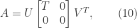
where 


The UTV decomposition is easy to update (when a row is added) and downdate (when a row is removed) using Givens rotations and it is suitable for parallel implementation. Initial determination of the UTV decomposition can be done by applying the updating algorithm as the rows are brought in one at a time.
LU Factorization
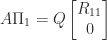
Instead of QR factorization we can build an RRF from an LU factorization with pivoting. For

where 


A result of Pan (2000) shows that an RRF based on LU factorization always exists up to a modest factor 
Theorem 3 For
![\notag \Pi_1 A \Pi_2 = LU = \begin{bmatrix} L_{11} & 0 \\ L_{12} & I_{m-k,n-k} \end{bmatrix} \begin{array}[b]{@{\mskip33mu}c@{\mskip-16mu}c@{\mskip-10mu}c@{}} \scriptstyle k & \scriptstyle n-k & \\ \multicolumn{2}{c}{ \left[\begin{array}{c@{~}c@{~}} U_{11}& U_{12} \\ 0 & U_{22} \\ \end{array}\right]} & \mskip-12mu\ \begin{array}{c} \scriptstyle k \\ \scriptstyle n-k \end{array} \end{array},](https://s0.wp.com/latex.php?latex=%5Cnotag+++++%5CPi_1+A+%5CPi_2+%3D+LU+%3D+++++%5Cbegin%7Bbmatrix%7D+++++L_%7B11%7D+%26++0++++%5C%5C+++++L_%7B12%7D+%26+I_%7Bm-k%2Cn-k%7D+++++%5Cend%7Bbmatrix%7D++++%5Cbegin%7Barray%7D%5Bb%5D%7B%40%7B%5Cmskip33mu%7Dc%40%7B%5Cmskip-16mu%7Dc%40%7B%5Cmskip-10mu%7Dc%40%7B%7D%7D++++%5Cscriptstyle+k+%26++++%5Cscriptstyle+n-k+%26++++%5C%5C++++%5Cmulticolumn%7B2%7D%7Bc%7D%7B++++++++%5Cleft%5B%5Cbegin%7Barray%7D%7Bc%40%7B%7E%7Dc%40%7B%7E%7D%7D++++++++++++++++++U_%7B11%7D%26+U_%7B12%7D+%5C%5C++++++++++++++++++++0+++%26+U_%7B22%7D+%5C%5C++++++++++++++%5Cend%7Barray%7D%5Cright%5D%7D++++%26+%5Cmskip-12mu%5C++++++++++%5Cbegin%7Barray%7D%7Bc%7D++++++++++++++%5Cscriptstyle+k+%5C%5C++++++++++++++%5Cscriptstyle+n-k++++++++++++++%5Cend%7Barray%7D++++%5Cend%7Barray%7D%2C+&bg=ffffff&fg=222222&s=0&c=20201002)
where

where
.
Again the proof is constructive, but the permutations it chooses are too expensive to compute. In practice, complete pivoting often yields a good RRF.
In terms of Definition 1, an RRF has

For the matrix (
U =
   1.0000e+00   1.0000e+00   1.0000e-08            0
            0  -2.0000e+00   2.0000e+00   1.0000e+00
            0            0   5.0000e-09  -1.5000e+00
            0            0            0  -2.0000e+00
As for QR factorization without pivoting, an RRF is not obtained from 
U =
   2.0000e+00   1.0000e+00  -1.0000e+00   1.0000e+00
            0  -2.0000e+00            0            0
            0            0   1.0000e+00   1.0000e+00
            0            0            0  -5.0000e-09
which yields a very good RRF 

Notes
QR factorization with column pivoting is difficult to implement efficiently, as the criterion for choosing the pivots requires the norms of the active parts of the remaining columns and this requires a significant amount of data movement. In recent years, randomized RRF algorithms have been developed that use projections with random matrices to make pivot decisions based on small sample matrices and thereby reduce the amount of data movement. See, for example, Martinsson et al. (2019).
References
This is a minimal set of references, which contain further useful references within.
- Shivkumar Chandrasekaran and Ilse C. F. Ipsen, On Rank-Revealing Factorisations, SIAM J. Matrix Anal. Appl. 15 (2), 592–622, 1994
- Y. P. Hong and C.-T. Pan, Rank-Revealing QR Factorizations and the Singular Value Decomposition, Math. Comp. 58 (197), 213–232, 1992.
- P. G. Martinsson, G. Quintana-Orti, and N. Heavner, randUTV: A Blocked Randomized Algorithm for Computing a Rank-Revealing UTV Factorization, ACM Trans. Math. Software 45(1), 4:1–4:26, 2019.
- C.-T. Pan, On the Existence and Computation of Rank-Revealing LU Factorizations, Linear Algebra Appl. 316, 199–222, 2000.
- G. W. Stewart, Matrix Algorithms. Volume I: Basic Decompositions, Society for Industrial and Applied Mathematics, Philadelphia, PA, USA, 1998.
Related Blog Posts
- What Is the CS Decomposition? (2020)
- What Is an LU Factorization? (2021)
- What Is a QR Factorization? (2020)
- What Is the Singular Value Decomposition? (2020)
This article is part of the “What Is” series, available from https://nhigham.com/category/what-is and in PDF form from the GitHub repository https://github.com/higham/what-is.
 is pseudo-orthogonal if
 is a signature matrix. A matrix
  -orthogonal matrix, where
  then
then  is also pseudo-orthogonal. Furthermore,
 is orthogonal, this equation implies that
  and hence that
 and
and ![\Sigma = \left[\begin{smallmatrix}1 & 0 \\ 0 & -1 \end{smallmatrix}\right]](https://s0.wp.com/latex.php?latex=%5CSigma+%3D+%5Cleft%5B%5Cbegin%7Bsmallmatrix%7D1+%26+0+%5C%5C+0+%26+-1+%5Cend%7Bsmallmatrix%7D%5Cright%5D&bg=ffffff&fg=222222&s=0&c=20201002) ,
, 

 matrices with
  .
. is an eigenvalue of
  is also an eigenvalue and it has the same algebraic and geometric multiplicities as
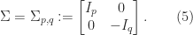
 , which means that
  , and any such orthogonal matrix is pseudo-orthogonal.
 of a symmetric positive definite
  and want the Cholesky factorization of
  , which is assumed to be symmetric positive definite. A more general downdating problem is that we are given
![\notag A = \begin{array}[b]{cc} \left[\begin{array}{@{}c@{}} A_1\\ A_2 \end{array}\right] & \mskip-22mu\ \begin{array}{l} \scriptstyle p \\ \scriptstyle q \end{array} \end{array}, \quad p\ge n,](https://s0.wp.com/latex.php?latex=%5Cnotag+++A+%3D+%5Cbegin%7Barray%7D%5Bb%5D%7Bcc%7D++++++++%5Cleft%5B%5Cbegin%7Barray%7D%7B%40%7B%7Dc%40%7B%7D%7D++++++++++++++++++A_1%5C%5C++++++++++++++++++A_2++++++++++++++%5Cend%7Barray%7D%5Cright%5D++++++++%26+%5Cmskip-22mu%5C++++++++++%5Cbegin%7Barray%7D%7Bl%7D++++++++++++++%5Cscriptstyle+p+%5C%5C++++++++++++++%5Cscriptstyle+q++++++++++%5Cend%7Barray%7D++++%5Cend%7Barray%7D%2C++++%5Cquad+p%5Cge+n%2C+&bg=ffffff&fg=222222&s=0&c=20201002)
 and wish to obtain the Cholesky factor
  of
of  . Note that
  have been removed. The simple case above corresponds to removing one row (
 ). Assuming that
  , we would like to obtain
  . If we can find a pseudo-orthogonal matrix
 upper triangular, then
 hyperbolic rotation has the form (4), and an
  hyperbolic rotation embedded in it at the intersection of rows and columns
  and
and  , for some
  and
and  has the form
 ![QA = \left[\begin{smallmatrix} R \\ 0 \end{smallmatrix}\right]](https://s0.wp.com/latex.php?latex=QA+%3D+%5Cleft%5B%5Cbegin%7Bsmallmatrix%7D+R+%5C%5C+0+%5Cend%7Bsmallmatrix%7D%5Cright%5D&bg=ffffff&fg=222222&s=0&c=20201002) with
with  and
and  upper triangular. The factorization exists if
  is positive definite.
 are given, and
  . For
. For  or
or  we have the standard least squares (LS) problem and the quadratic form is definite, while for
  the problem is to minimize a genuinely indefinite quadratic form. This problem arises, for example, in the area of optimization known as
  smoothing.
 , and since the Hessian matrix of the quadratic objective function in (7) is
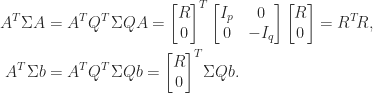
 , where
  comprises the first
  components of
  . The same equation can also be obtained without using the normal equations by substituting the hyperbolic QR factorization into (7).
 with
with  , partition
![\notag A = \mskip5mu \begin{array}[b]{@{\mskip-20mu}c@{\mskip0mu}c@{\mskip-1mu}c@{}} & \mskip10mu\scriptstyle p & \scriptstyle q \\ \mskip15mu \begin{array}{r} \scriptstyle p \\ \scriptstyle q \end{array}~ & \multicolumn{2}{c}{\mskip-15mu \left[\begin{array}{c@{~}c@{~}} A_{11} & A_{12}\\ A_{21} & A_{22} \end{array}\right] } \end{array}, \qquad (8)](https://s0.wp.com/latex.php?latex=%5Cnotag+++A++%3D+%5Cmskip5mu++++%5Cbegin%7Barray%7D%5Bb%5D%7B%40%7B%5Cmskip-20mu%7Dc%40%7B%5Cmskip0mu%7Dc%40%7B%5Cmskip-1mu%7Dc%40%7B%7D%7D++++%26+%5Cmskip10mu%5Cscriptstyle+p+%26+%5Cscriptstyle+q+%5C%5C+++++++%5Cmskip15mu++++++++++%5Cbegin%7Barray%7D%7Br%7D++++++++++++++%5Cscriptstyle+p+%5C%5C++++++++++++++%5Cscriptstyle+q++++++++++%5Cend%7Barray%7D%7E++++%26+++++++%5Cmulticolumn%7B2%7D%7Bc%7D%7B%5Cmskip-15mu++++++++++%5Cleft%5B%5Cbegin%7Barray%7D%7Bc%40%7B%7E%7Dc%40%7B%7E%7D%7D++++++++++++++++++A_%7B11%7D+%26+A_%7B12%7D%5C%5C++++++++++++++++++A_%7B21%7D+%26+A_%7B22%7D++++++++++++++++%5Cend%7Barray%7D%5Cright%5D+++++++%7D++++%5Cend%7Barray%7D%2C+%5Cqquad+%288%29+&bg=ffffff&fg=222222&s=0&c=20201002)
 is nonsingular. The exchange operator is defined by
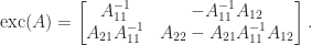


 .
. exists then
  .
.
 and then eliminating
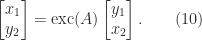
 , we have
 there is a unique
  and
and  , which implies by (10) that
  , which implies that
  , it follows that
  also has a nonsingular
  block and so
  . But (9) shows that
  , and we conclude that
  exists and Lemma 1 shows that
  . Hence, using (9),
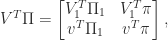
 be pseudo-orthogonal with respect to
 ![\notag Q = \begin{array}[b]{@{\mskip33mu}c@{\mskip-16mu}c@{\mskip-10mu}c@{}} \scriptstyle p & \scriptstyle n-p & \\ \multicolumn{2}{c}{ \left[\begin{array}{c@{~}c@{~}} Q_{11}& Q_{12} \\ Q_{21}& Q_{22} \\ \end{array}\right]} & \mskip-12mu\ \begin{array}{c} \scriptstyle p \\ \scriptstyle n-p \end{array} \end{array}, \quad p \le \displaystyle\frac{n}{2}.](https://s0.wp.com/latex.php?latex=%5Cnotag++++Q+%3D++++%5Cbegin%7Barray%7D%5Bb%5D%7B%40%7B%5Cmskip33mu%7Dc%40%7B%5Cmskip-16mu%7Dc%40%7B%5Cmskip-10mu%7Dc%40%7B%7D%7D++++%5Cscriptstyle+p+%26++++%5Cscriptstyle+n-p+%26++++%5C%5C++++%5Cmulticolumn%7B2%7D%7Bc%7D%7B++++++++%5Cleft%5B%5Cbegin%7Barray%7D%7Bc%40%7B%7E%7Dc%40%7B%7E%7D%7D++++++++++++++++++Q_%7B11%7D%26+Q_%7B12%7D+%5C%5C++++++++++++++++++Q_%7B21%7D%26+Q_%7B22%7D+%5C%5C++++++++++++++%5Cend%7Barray%7D%5Cright%5D%7D++++%26+%5Cmskip-12mu%5C++++++++++%5Cbegin%7Barray%7D%7Bc%7D++++++++++++++%5Cscriptstyle+p+%5C%5C++++++++++++++%5Cscriptstyle+n-p++++++++++++++%5Cend%7Barray%7D++++%5Cend%7Barray%7D%2C+%5Cquad+p+%5Cle+%5Cdisplaystyle%5Cfrac%7Bn%7D%7B2%7D.+&bg=ffffff&fg=222222&s=0&c=20201002)
 and
and  such that
![\notag \begin{bmatrix} U_1^T & 0\\ 0 & U_2^T \end{bmatrix} \begin{bmatrix} Q_{11} & Q_{12}\\ Q_{21} & Q_{22} \end{bmatrix} \begin{bmatrix} V_1 & 0\\ 0 & V_2 \end{bmatrix} = \begin{array}[b]{@{\mskip35mu}c@{\mskip30mu}c@{\mskip-10mu}c@{}c} \scriptstyle p & \scriptstyle p & \scriptstyle n-2p & \\ \multicolumn{3}{c}{ \left[\begin{array}{c@{~}|c@{~}c} C & -S & 0 \\ \hline -S & C & 0 \\ 0 & 0 & I_{n-2p} \end{array}\right]} & \mskip-12mu \begin{array}{c} \scriptstyle p \\ \scriptstyle p \\ \scriptstyle n-2p \end{array} \end{array}, \qquad (11)](https://s0.wp.com/latex.php?latex=%5Cnotag++++%5Cbegin%7Bbmatrix%7D++U_1%5ET+%26+0%5C%5C++++++++++++++++++++++++++0+++%26+U_2%5ET++++%5Cend%7Bbmatrix%7D++++%5Cbegin%7Bbmatrix%7D++Q_%7B11%7D+%26+Q_%7B12%7D%5C%5C++++++++++++++++++++++++++Q_%7B21%7D+%26+Q_%7B22%7D++++%5Cend%7Bbmatrix%7D++++%5Cbegin%7Bbmatrix%7D++V_1+%26+0%5C%5C++++++++++++++++++++++++++0+++%26+V_2++++%5Cend%7Bbmatrix%7D++++%3D++++%5Cbegin%7Barray%7D%5Bb%5D%7B%40%7B%5Cmskip35mu%7Dc%40%7B%5Cmskip30mu%7Dc%40%7B%5Cmskip-10mu%7Dc%40%7B%7Dc%7D++++%5Cscriptstyle+p+%26++++%5Cscriptstyle+p+%26++++%5Cscriptstyle+n-2p+%26++++%5C%5C++++%5Cmulticolumn%7B3%7D%7Bc%7D%7B++++%5Cleft%5B%5Cbegin%7Barray%7D%7Bc%40%7B%7E%7D%7Cc%40%7B%7E%7Dc%7D++++C+%26+++-S++++++%26+0+++%5C%5C++++%5Chline+++-S+%26++++C++++++%26+0+++%5C%5C++++0+%26++++0++++++%26+I_%7Bn-2p%7D++++%5Cend%7Barray%7D%5Cright%5D%7D++++%26+%5Cmskip-12mu++++%5Cbegin%7Barray%7D%7Bc%7D++++%5Cscriptstyle+p+%5C%5C++++%5Cscriptstyle+p+%5C%5C++++%5Cscriptstyle+n-2p++++%5Cend%7Barray%7D++++%5Cend%7Barray%7D%2C+%5Cqquad+%2811%29+&bg=ffffff&fg=222222&s=0&c=20201002)
 ,
,  , and
, and  , with
  for all
  .
.![\left[\begin{smallmatrix}C & -S \\ -S & C \end{smallmatrix}\right]](https://s0.wp.com/latex.php?latex=%5Cleft%5B%5Cbegin%7Bsmallmatrix%7DC+%26+-S+%5C%5C+-S+%26+C+%5Cend%7Bsmallmatrix%7D%5Cright%5D&bg=ffffff&fg=222222&s=0&c=20201002) in (11) generalizes the
in (11) generalizes the 
 for all
  singular values occur in reciprocal pairs, hence the largest and smallest singular values satisfy
  (with strict inequality unless
  ). This gives another proof of (3).
 for
for  . More results for pseudo-orthogonal matrices can be obtained as special cases of results for automorphism groups of general scalar products. See, for example, Mackey, Mackey, and Tisseur (2006).
 the set of pseudo-orthogonal matrices is known to have four connected components, a topological property that can be proved using the hyperbolic CS decomposition (Motlaghian, Armandnejad, and Hall, 2018).
 such that
  . These correspond to the automorphism group of the scalar product
  for
for  . The results we have discussed generalize in a straightforward way to pseudo-unitary matrices.
 , where
 ![\notag \left[\begin{array}{rrrr} 3 & -1 & 1 & 1\\ -1 & 3 & 1 & -1\\ -1 & -1 & 3 & 1\\ 1 & 1 & 1 & 3 \end{array}\right] = \left[\begin{array}{rrrr} 1 & 0 & 0 & 0\\ -\frac{1}{3} & 1 & 0 & 0\\ -\frac{1}{3} & -\frac{1}{2} & 1 & 0\\ \frac{1}{3} & \frac{1}{2} & 0 & 1 \end{array}\right] \left[\begin{array}{rrrr} 3 & -1 & 1 & 1\\ 0 & \frac{8}{3} & \frac{4}{3} & -\frac{2}{3}\\ 0 & 0 & 4 & 1\\ 0 & 0 & 0 & 3 \end{array}\right]. \qquad (1)](https://s0.wp.com/latex.php?latex=%5Cnotag++++%5Cleft%5B%5Cbegin%7Barray%7D%7Brrrr%7D++++++3+%26+-1+%26+1+%26+1%5C%5C+++++-1+%26+3+%26+1+%26+-1%5C%5C+++++-1+%26+-1+%26+3+%26+1%5C%5C++++++1+%26+1+%26+1+%26+3++++%5Cend%7Barray%7D%5Cright%5D+++%3D++++%5Cleft%5B%5Cbegin%7Barray%7D%7Brrrr%7D+++++1+%26+0+%26+0+%26+0%5C%5C++++-%5Cfrac%7B1%7D%7B3%7D+%26+1+%26+0+%26+0%5C%5C++++-%5Cfrac%7B1%7D%7B3%7D+%26+-%5Cfrac%7B1%7D%7B2%7D+%26+1+%26+0%5C%5C+++++%5Cfrac%7B1%7D%7B3%7D+%26+%5Cfrac%7B1%7D%7B2%7D+%26+0+%26+1++++%5Cend%7Barray%7D%5Cright%5D++++%5Cleft%5B%5Cbegin%7Barray%7D%7Brrrr%7D++++3+%26+-1+%26+1+%26+1%5C%5C++++0+%26+%5Cfrac%7B8%7D%7B3%7D+%26+%5Cfrac%7B4%7D%7B3%7D+%26+-%5Cfrac%7B2%7D%7B3%7D%5C%5C++++0+%26+0+%26+4+%26+1%5C%5C++++0+%26+0+%26+0+%26+3++++%5Cend%7Barray%7D%5Cright%5D.+%5Cqquad+%281%29+&bg=ffffff&fg=222222&s=0&c=20201002)
 reduces to solving the triangular systems
  and
and  , since then
  .
. the leading principal submatrix of
  . If
. If  then the factorization may exist, but if so it is not unique.
 then the
  are necessarily nonsingular and so
  . The left side of this equation is unit lower triangular and the right side is upper triangular; therefore both sides must equal the identity matrix, which means that
  and
and  , as required.
 , which implies that
  . Hence
  . In fact, such determinantal formulas hold for all the elements of
 ![\notag \begin{aligned} \ell_{ij} &= \frac{ \det\bigl( A( [1:j-1, \, i], 1:j ) \bigr) }{ \det( A_j ) }, \quad i > j, \\ u_{ij} &= \frac{ \det\bigl( A( 1:i, [1:i-1, \, j] ) \bigr) } { \det( A_{i-1} ) }, \quad i \le j. \end{aligned}](https://s0.wp.com/latex.php?latex=%5Cnotag++++%5Cbegin%7Baligned%7D++++%5Cell_%7Bij%7D+%26%3D+%5Cfrac%7B+%5Cdet%5Cbigl%28+A%28+%5B1%3Aj-1%2C+%5C%2C+i%5D%2C+1%3Aj+%29+%5Cbigr%29+%7D%7B+%5Cdet%28+A_j+%29+%7D%2C+++++++++++++%5Cquad+i+%3E+j%2C+%5C%5C++++u_%7Bij%7D+%26%3D+%5Cfrac%7B+%5Cdet%5Cbigl%28+A%28+1%3Ai%2C+%5B1%3Ai-1%2C+%5C%2C+j%5D+%29+%5Cbigr%29+%7D+++++++++++++++++++%7B+%5Cdet%28+A_%7Bi-1%7D+%29+%7D%2C+++++++++++++%5Cquad+i+%5Cle+j.++++%5Cend%7Baligned%7D+&bg=ffffff&fg=222222&s=0&c=20201002)
 , where
  and
and  are vectors of subscripts, denotes the submatrix formed from the intersection of the rows indexed by
  to upper triangular form
  in
in  stages. At the
 are the multipliers. Of course each
  must be nonzero for these formulas to be defined, and this is connected with the conditions of Theorem 1, since
  . The final
  for
for  , and
, and  for
for  , that is, the multipliers make up the
  we can just solve
  and
and  , re-using the LU factorization. Similarly, solving
  reduces to solving the triangular systems
  and
and  .
. then determines the first column of
  . This leads to the Doolittle method, which involves inner products of partial rows of
 ordering of the loops in the factorization is the basis of early Fortran implementations of LU factorization, such as that in LINPACK. The inner loop travels down the columns of
  ordering, which updates the matrix a row at a time, and is appropriate for a language such as C that stores arrays by row.
 and
and  orderings correspond to the Doolittle method. The last two of the
  orderings are the
  and
and  orderings, to which we will return later.
 we can write
 matrix
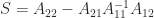
  is called the Schur complement of
  in
in  and
and  have the correct forms for a unit lower triangular matrix and an upper triangular matrix, respectively. If we can find an LU factorization
  then
then
 . If we can show that the Schur complement inherits the same structure then it follows by induction that we can compute the factorization for
  and
and  -matrices,
 if
if  for
for  and lower bandwidth
  if
if  . Another use of (2) is to show that
  and
and  have only
  :
:
 . This leads to the following algorithm:
 .
. for
for  .
. for
for  .
. .
. .
. partitioning, in which we assume we have already computed the first block column of
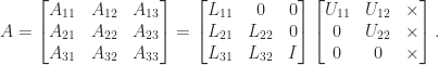
 .
. for
for  .
. —
— .
. lower triangular and
  , where
![\notag A = \left[ \begin{array}{rr|rr} 0 & 1 & 1 & 1 \\ -1 & 1 & 1 & 1 \\\hline -2 & 3 & 4 & 2 \\ -1 & 2 & 1 & 3 \\ \end{array} \right] = \left[ \begin{array}{cc|cc} 1 & 0 & 0 & 0 \\ 0 & 1 & 0 & 0 \\\hline 1 & 2 & 1 & 0 \\ 1 & 1 & 0 & 1 \\ \end{array} \right] \left[ \begin{array}{rr|rr} 0 & 1 & 1 & 1 \\ -1 & 1 & 1 & 1 \\\hline 0 & 0 & 1 & -1 \\ 0 & 0 & -1 & 1 \\ \end{array} \right].](https://s0.wp.com/latex.php?latex=%5Cnotag+++++A+%3D++++++%5Cleft%5B+%5Cbegin%7Barray%7D%7Brr%7Crr%7D++++++0++%26++1++%26++1++%26++1++%5C%5C+++++-1++%26++1++%26++1++%26++1++%5C%5C%5Chline+++++-2++%26++3++%26++4++%26++2++%5C%5C+++++-1++%26++2++%26++1++%26++3++%5C%5C+++++++++++++%5Cend%7Barray%7D++++++%5Cright%5D++++++%3D++++++%5Cleft%5B+%5Cbegin%7Barray%7D%7Bcc%7Ccc%7D++++++1++%26++0++%26++0++%26++0++%5C%5C++++++0++%26++1++%26++0++%26++0++%5C%5C%5Chline++++++1++%26++2++%26++1++%26++0++%5C%5C++++++1++%26++1++%26++0++%26++1++%5C%5C+++++++++++++%5Cend%7Barray%7D++++++%5Cright%5D++++++%5Cleft%5B+%5Cbegin%7Barray%7D%7Brr%7Crr%7D++++++0++%26++1++%26++1++%26++1++%5C%5C+++++-1++%26++1++%26++1++%26++1++%5C%5C%5Chline++++++0++%26++0++%26++1++%26+-1++%5C%5C++++++0++%26++0++%26+-1++%26++1++%5C%5C+++++++++++++%5Cend%7Barray%7D++++++%5Cright%5D.+&bg=ffffff&fg=222222&s=0&c=20201002)
 submatrix. In the context of a linear system
  , we have effectively solved for the variables
  and
and  and then substituted for
  leading principal block submatrices of
  involving the diagonal blocks of
  an LU factorization
  exists. To first order, this equation is
  , which gives
 is strictly lower triangular and
  is upper triangular, we have, to first order,
 denotes the strictly lower triangular part and
  the strictly upper triangular part. Clearly, the sensitivity of the LU factors depends on the inverses of
  and
and  are numerically stable in the sense that
  with
with  , where
  is a constant and
![\notag \left[\begin{array}{rrr} 3 & -1 & -2\\ -2 & 3 & -1\\ -2 & -1 & 3 \end{array}\right] \qquad (1)](https://s0.wp.com/latex.php?latex=%5Cnotag++%5Cleft%5B%5Cbegin%7Barray%7D%7Brrr%7D+++++3+%26+-1+%26+-2%5C%5C++++-2+%26++3+%26+-1%5C%5C++++-2+%26+-1+%26++3+++%5Cend%7Barray%7D%5Cright%5D+%5Cqquad+%281%29+&bg=ffffff&fg=222222&s=0&c=20201002)
![[1~1~1]^T](https://s0.wp.com/latex.php?latex=%5B1%7E1%7E1%5D%5ET&bg=ffffff&fg=222222&s=0&c=20201002) is a null vector. A useful definition of a matrix with large diagonal requires a stronger property.
is a null vector. A useful definition of a matrix with large diagonal requires a stronger property. is diagonally dominant by rows if
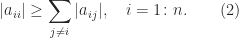
 is (strictly) diagonally dominant by rows.
 let
let  and choose
  . Then the

 and so
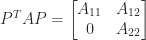
 square matrices. Irreducibility is equivalent to the directed graph of
  for some
  such that
  . Define

 ,
,
 is nonempty, because if it were empty then we would have
  for all
  , then putting
  , which is a contradiction. Hence as long as
  for some
  , we obtain
  , which contradicts the diagonal dominance. Therefore we must have
  for all
  . This means that all the rows indexed by
  have zeros in the columns indexed by
 ![\notag T_n = \left[\begin{array}{@{\mskip 5mu}c*{4}{@{\mskip 15mu} r}@{\mskip 5mu}} 2 & -1 & & & \\ -1 & 2 & -1 & & \\ & -1 & 2 & \ddots & \\ & & \ddots & \ddots & -1\\ & & & -1 & 2 \end{array}\right], \qquad (5)](https://s0.wp.com/latex.php?latex=%5Cnotag++T_n+%3D+%5Cleft%5B%5Cbegin%7Barray%7D%7B%40%7B%5Cmskip+5mu%7Dc%2A%7B4%7D%7B%40%7B%5Cmskip+15mu%7D+r%7D%40%7B%5Cmskip+5mu%7D%7D++++++2+%26+++-1++%26++++++++++%26+++++++++%26+%5C%5C+++++-1+%26++++2++%26++-1++++++%26+++++++++%26+%5C%5C++++++++%26++++-1+%26+++2++++++%26++%5Cddots+%26+%5C%5C++++++++%26+++++++%26++%5Cddots++%26++%5Cddots+%26+-1%5C%5C++++++++%26+++++++%26++++++++++%26++-1+++++%26+2++++++++++++%5Cend%7Barray%7D%5Cright%5D%2C+%5Cqquad+%285%29+&bg=ffffff&fg=222222&s=0&c=20201002)
 or
or  by
by 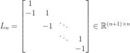
 and
and
 and
and  have the same nonzero eigenvalues, we conclude that
  , where
  denotes the spectrum. Hence
  is symmetric positive definite and
  is singular and symmetric positive semidefinite.
 is singular and hence cannot be strictly diagonally dominant, by Theorem 1. So
 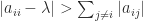 cannot be true for all
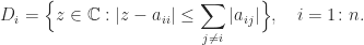
 , so
, so  , so the eigenvalues are nonnegative, and hence positive since nonzero. This provides another proof that the matrix

 is diagonally dominant by rows for some diagonal matrix
  with
with  for all
 , defined by
 partitioning
  , the diagonal blocks
  are all nonsingular and
 then block diagonal dominance reduces to the usual notion of diagonal dominance. Block diagonal dominance holds for certain block tridiagonal matrices arising in the discretization of PDEs.
 .
. . Let
. Let  satisfy
  and let
  . The result is obtained on applying this bound to
  .
.  , where
  ,
,  , and
, and  for
for  . It is easy to see that
  , which gives another proof that
 , so in view of its sign pattern
  .
.
 .
. satisfies
  for all
  . Let
. Let  . Taking absolute values in
  gives
gives
 , since
  . This inequality holds for all
  , which gives the result.
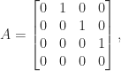
 is an upper Hessenberg matrix of the form
 can be transposed and permuted so that the coefficients
  appear in the first or last column or the last row. By expanding the determinant about the first row it can be seen that
 add
add  times the
  , to obtain
  as the new last column, and expand the determinant about the last column.) MacDuffee (1946) introduced the term “companion matrix” as a translation from the German “Begleitmatrix”.
 in
in  , so
, so  . The inverse is
 is in companion form, where
  is the reverse identity matrix, and the coefficients are those of the polynomial
  , whose roots are the reciprocals of those of
 differs from
  , where
  is a rank-
![[\lambda^{n-1}, \lambda^{n-2}, \dots, \lambda, 1]^T](https://s0.wp.com/latex.php?latex=%5B%5Clambda%5E%7Bn-1%7D%2C+%5Clambda%5E%7Bn-2%7D%2C+%5Cdots%2C+%5Clambda%2C+1%5D%5ET&bg=ffffff&fg=222222&s=0&c=20201002) is a corresponding eigenvector. The last
is a corresponding eigenvector. The last ![[p_1,p_2, \dots, p_{n+1}]](https://s0.wp.com/latex.php?latex=%5Bp_1%2Cp_2%2C+%5Cdots%2C+p_%7Bn%2B1%7D%5D&bg=ffffff&fg=222222&s=0&c=20201002) of the coefficients of a polynomial,
of the coefficients of a polynomial,  , and returns the companion matrix with
  , …,
, …,  .
.
 . These formulae generalize to block companion matrices, as shown by Higham and Tisseur (2003).
 ,
,  , which satisfy the recurrence
  for
for  , with
  . We can write
![\left[\begin{smallmatrix}1 & 1 \\ 1 & 0 \end{smallmatrix}\right]](https://s0.wp.com/latex.php?latex=%5Cleft%5B%5Cbegin%7Bsmallmatrix%7D1+%26+1+%5C%5C+1+%26+0+%5Cend%7Bsmallmatrix%7D%5Cright%5D&bg=ffffff&fg=222222&s=0&c=20201002) is a companion matrix. This expression can be used to compute
is a companion matrix. This expression can be used to compute  in
in  operations by computing the matrix power using binary powering.
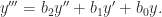


 storage instead of the
  storage that should be possible given the structure of
  for some
  with
with  . It is not necessarily the case that the computed roots are the exact roots of a polynomial with coefficients
  with
with  for all

 denote the field
  or
or  .
. then
then  where
where  is nonsingular and
  , with each
  a companion matrix.
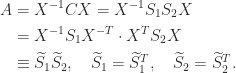
 is nonsingular, and since
  can alternatively be taken nonsingular by considering the factorization of
  , either one of which can be taken nonsingular, such that
  .
. with the
  symmetric then
  , so
, so  is symmetric. Likewise,
  is symmetric.
 similar to
  it is
it is![\notag \widetilde{C} = \begin{bmatrix} a_4 & a_3 & 1 & 0 & 0 \\ 1 & 0 & 0 & 0 & 0 \\ 0 & a_2 & 0 & a_1 & 1 \\ 0 & 1 & 0 & 0 & 0 \\ 0 & 0 & 0 & a_0 & 0 \end{bmatrix} = \left[\begin{array}{cc|cc|c} a_4 & 1 & & & \\ 1 & 0 & & & \\\hline & & a_2 & 1 & \\ & & 1 & 0 & \\\hline & & & & a_0 \end{array}\right] \left[\begin{array}{c|cc|cc} 1 & & & & \\\hline & a_3 & 1 & & \\ & 1 & 0 & & \\\hline & & & a_1 & 1 \\ & & & 1 & 0 \end{array}\right].](https://s0.wp.com/latex.php?latex=%5Cnotag+%5Cwidetilde%7BC%7D+%3D+%5Cbegin%7Bbmatrix%7D++++a_4+%26+a_3+%26+1++%26+0+++%26+0++%5C%5C++++++1+%26+0+++%26+0++%26+0+++%26+0++%5C%5C++++++0+%26+a_2+%26+0++%26+a_1+%26+1++%5C%5C++++++0+%26+1+++%26+0++%26+0+++%26+0+%5C%5C++++++0+%26+0+++%26+0++%26+a_0+%26+0+%5Cend%7Bbmatrix%7D+%3D+%5Cleft%5B%5Cbegin%7Barray%7D%7Bcc%7Ccc%7Cc%7D++++a_4+%26+1+%26+++++%26+++%26+++%5C%5C++++++1+%26+0+%26+++++%26+++%26+++%5C%5C%5Chline++++++++%26+++%26+a_2+%26+1+%26+++%5C%5C++++++++%26+++%26++1++%26+0+%26+++%5C%5C%5Chline++++++++%26+++%26+++++%26+++%26++a_0+%5Cend%7Barray%7D%5Cright%5D+%5Cleft%5B%5Cbegin%7Barray%7D%7Bc%7Ccc%7Ccc%7D++++++1++%26+++++%26+++%26++++++%26+%5C%5C%5Chline+++++++++%26+a_3+%26+1+%26++++++%26+%5C%5C+++++++++%26++1++%26+0+%26++++++%26+%5C%5C%5Chline+++++++++%26+++++%26+++%26++a_1+%26+1+%5C%5C+++++++++%26+++++%26+++%26+++1++%26+0+%5Cend%7Barray%7D%5Cright%5D.+&bg=ffffff&fg=222222&s=0&c=20201002)
 , by taking the
  -norm of the companion matrix
 of the form
 is the spectral radius of
  , that is, the largest modulus of any eigenvalue of
  denotes that

 , we can set it to
  . Indeed let
  and
and  . Then
  , since
  and
and  for
for  . Furthermore, for a nonnegative matrix the spectral radius is an eigenvalue, by the Perron–Frobenius theorem, so
  is an eigenvalue of
  . Hence
  .
. satisfies
  ,
,

 is an
is an  .
.![\notag T_4 = \left[\begin{array}{@{\mskip 5mu}c*{3}{@{\mskip 15mu} r}@{\mskip 5mu}} 1 & -1 & -1 & -1 \\ & 1 & -1 & -1 \\ & & 1 & -1 \\ & & & 1 \end{array}\right], \quad T_4^{-1} = \begin{bmatrix} 1 & 1 & 2 & 4\\ & 1 & 1 & 2\\ & & 1 & 1\\ & & & 1 \end{bmatrix}.](https://s0.wp.com/latex.php?latex=%5Cnotag+++++T_4+%3D+%5Cleft%5B%5Cbegin%7Barray%7D%7B%40%7B%5Cmskip+5mu%7Dc%2A%7B3%7D%7B%40%7B%5Cmskip+15mu%7D+r%7D%40%7B%5Cmskip+5mu%7D%7D++++++1+%26+++-1++%26++-1++%26+-1+%5C%5C++++++++%26++++1++%26++-1++%26+-1+%5C%5C++++++++%26+++++++%26+++1++%26+-1+%5C%5C++++++++%26+++++++%26++++++%26++1++++++++++++%5Cend%7Barray%7D%5Cright%5D%2C+%5Cquad+++T_4%5E%7B-1%7D+%3D++++%5Cbegin%7Bbmatrix%7D++++1+%26+1+%26+2+%26+4%5C%5C+++%26+1+%26+1+%26+2%5C%5C+++%26+++%26+1+%26+1%5C%5C+++%26+++%26+++%26+1++++%5Cend%7Bbmatrix%7D.+&bg=ffffff&fg=222222&s=0&c=20201002)
 is the matrix
 is an
is an 
 denoting the vector of ones, since
  is nonnegative we have
 can be computed in
  costs
costs  of an
of an 
 , which follows from
  with the same
  by
by![\notag A_4 = \left[\begin{array}{@{\mskip 5mu}c*{3}{@{\mskip 15mu} r}@{\mskip 5mu}} 2 & -1 & & \\ -1 & 2 & -1 & \\ & -1 & 2 & -1 \\ & & -1 & 2 \end{array}\right], \quad A_4^{-1} = \begin{bmatrix} \frac{4}{5} & \frac{3}{5} & \frac{2}{5} & \frac{1}{5}\\[\smallskipamount] \frac{3}{5} & \frac{6}{5} & \frac{4}{5} & \frac{2}{5}\\[\smallskipamount] \frac{2}{5} & \frac{4}{5} & \frac{6}{5} & \frac{3}{5}\\[\smallskipamount] \frac{1}{5} & \frac{2}{5} & \frac{3}{5} & \frac{4}{5} \end{bmatrix}.](https://s0.wp.com/latex.php?latex=%5Cnotag+++++A_4+%3D+%5Cleft%5B%5Cbegin%7Barray%7D%7B%40%7B%5Cmskip+5mu%7Dc%2A%7B3%7D%7B%40%7B%5Cmskip+15mu%7D+r%7D%40%7B%5Cmskip+5mu%7D%7D++++++2+%26+++-1++%26++++++%26++++%5C%5C+++++-1+%26++++2++%26++-1++%26++++%5C%5C++++++++%26++++-1+%26+++2++%26++-1+%5C%5C++++++++%26+++++++%26++-1++%26++2++++++++++++%5Cend%7Barray%7D%5Cright%5D%2C+%5Cquad+++A_4%5E%7B-1%7D+%3D++++%5Cbegin%7Bbmatrix%7D+++%5Cfrac%7B4%7D%7B5%7D+%26+%5Cfrac%7B3%7D%7B5%7D+%26+%5Cfrac%7B2%7D%7B5%7D+%26+%5Cfrac%7B1%7D%7B5%7D%5C%5C%5B%5Csmallskipamount%5D+++%5Cfrac%7B3%7D%7B5%7D+%26+%5Cfrac%7B6%7D%7B5%7D+%26+%5Cfrac%7B4%7D%7B5%7D+%26+%5Cfrac%7B2%7D%7B5%7D%5C%5C%5B%5Csmallskipamount%5D+++%5Cfrac%7B2%7D%7B5%7D+%26+%5Cfrac%7B4%7D%7B5%7D+%26+%5Cfrac%7B6%7D%7B5%7D+%26+%5Cfrac%7B3%7D%7B5%7D%5C%5C%5B%5Csmallskipamount%5D+++%5Cfrac%7B1%7D%7B5%7D+%26+%5Cfrac%7B2%7D%7B5%7D+%26+%5Cfrac%7B3%7D%7B5%7D+%26+%5Cfrac%7B4%7D%7B5%7D+%5Cend%7Bbmatrix%7D.+&bg=ffffff&fg=222222&s=0&c=20201002)
![\notag A = \begin{array}[b]{@{\mskip27mu}c@{\mskip-20mu}c@{\mskip-10mu}c@{}} \scriptstyle 1 & \scriptstyle n-1 & \\ \multicolumn{2}{c}{ \left[\begin{array}{c@{~}c@{~}} \alpha & b^T \\ c^T & E \\ \end{array}\right]} & \mskip-14mu\ \begin{array}{c} \scriptstyle 1 \\ \scriptstyle n-1 \end{array} \end{array}, \quad \alpha > 0, \quad b\le 0, \quad c \le 0.](https://s0.wp.com/latex.php?latex=%5Cnotag++++A+%3D++++%5Cbegin%7Barray%7D%5Bb%5D%7B%40%7B%5Cmskip27mu%7Dc%40%7B%5Cmskip-20mu%7Dc%40%7B%5Cmskip-10mu%7Dc%40%7B%7D%7D++++%5Cscriptstyle+1+%26++++%5Cscriptstyle+n-1+%26++++%5C%5C++++%5Cmulticolumn%7B2%7D%7Bc%7D%7B++++++++%5Cleft%5B%5Cbegin%7Barray%7D%7Bc%40%7B%7E%7Dc%40%7B%7E%7D%7D++++++++++++++++++%5Calpha+%26+b%5ET+%5C%5C++++++++++++++++++c%5ET++++%26+E++%5C%5C++++++++++++++%5Cend%7Barray%7D%5Cright%5D%7D++++%26+%5Cmskip-14mu%5C++++++++++%5Cbegin%7Barray%7D%7Bc%7D++++++++++++++%5Cscriptstyle+1+%5C%5C++++++++++++++%5Cscriptstyle+n-1++++++++++++++%5Cend%7Barray%7D++++%5Cend%7Barray%7D%2C+++%5Cquad+%5Calpha+%3E+0%2C+%5Cquad+b%5Cle+0%2C+%5Cquad+c+%5Cle+0.+&bg=ffffff&fg=222222&s=0&c=20201002)


 . It is easy to see that
  , and hence Theorem
  is strictly diagonally dominant by columns for some diagonal matrix
  for all
 because of the sign pattern of
  , and partial pivoting does not require row interchanges. The effect of row scaling on LU factorization is easy to see:
 is unit lower triangular, so that
  are the LU factors of
![\notag A^{-1} = \begin{bmatrix} \displaystyle\frac{1}{\epsilon}& 0& \displaystyle\frac{1}{\epsilon}\\[\bigskipamount] \displaystyle\frac{1}{\epsilon}& 1 & \displaystyle\frac{1 + \epsilon}{\epsilon}\\[\bigskipamount] 0& 0& 1 \end{bmatrix} \ge 0,](https://s0.wp.com/latex.php?latex=%5Cnotag++A%5E%7B-1%7D+%3D++++%5Cbegin%7Bbmatrix%7D++++++++%5Cdisplaystyle%5Cfrac%7B1%7D%7B%5Cepsilon%7D%26+0%26+%5Cdisplaystyle%5Cfrac%7B1%7D%7B%5Cepsilon%7D%5C%5C%5B%5Cbigskipamount%5D++++++++%5Cdisplaystyle%5Cfrac%7B1%7D%7B%5Cepsilon%7D%26+1+%26+%5Cdisplaystyle%5Cfrac%7B1+%2B+%5Cepsilon%7D%7B%5Cepsilon%7D%5C%5C%5B%5Cbigskipamount%5D++++++++++++++++++0%26+++++++++++0%26+++++1++++%5Cend%7Bbmatrix%7D+%5Cge+0%2C+&bg=ffffff&fg=222222&s=0&c=20201002)
 element of the LU factor
  , which means that
 is large, in that the computed LU factors have a large relative residual. We conclude that pivoting is necessary for numerical stability in LU factorization of
  with
with  . This iteration converges for all starting vectors
  if
if  . Much interest has focused on regular splittings, which are defined as ones for which
  and
and  . An
. An  ) are all convergent for
  of an
of an 
 in
in  . A nonnegative vector
  such that
  is called a stationary distribution vector and is of interest for describing the properties of the Markov chain. To compute
  . Clearly,
  , so
, so  Decompositions of Generalized Diagonally Dominant Matrices
 is unitarily invariant if
  for all unitary
  and
and  and for all
  . One can restrict the definition to real matrices, though the term unitarily invariant is still typically used.
 , using the fact that
  , we obtain
 ,
,

 , so
, so  depends only on the singular values. Indeed, for the 2-norm and the Frobenius norm we have
  and
and  . Here, and throughout this article,
  . Another implication of the singular value dependence is that
  for all
  such that
  is an absolute norm on
  and
and  for any permutation matrix
  for all
  implies
  for all
  for all
  are the singular values of
 , which is called the trace norm or nuclear norm. It can act as a proxy for the rank of a matrix. The trace norm can be expressed as
  , where
  is a polar decomposition.
 and
and  .
. is the
  (
( have SVDs with diagonal matrices
  , where the diagonal elements are arranged in nonincreasing order. Then
  for every unitarily invariant norm.
 is defined,
 for all
  if and only if
  for all
  for all
  if and only if the norm is a positive scalar multiple of the Frobenius norm.
 , what is the nearest symmetric matrix whose eigenvalues are all at least
  .
. , the problem arises when the matrix is positive definite but ill conditioned and a matrix of smaller condition number is required, or when rounding errors result in small negative eigenvalues and a “safely positive definite” matrix is wanted.
 and let
  . The unique matrix with smallest eigenvalue at least
 , another way to express this result is in terms of the polar decomposition
  , since
  .
.
 to denote that the symmetric matrix
  to denote the positive semidefinite square root.


 , the nearest matrix and the distance reduce to
 we could just perturb the negative eigenvalue to zero, as with the optimal Frobenius norm perturbation, without changing the
  for any other nearest positive semidefinite matrix
  is an approximate minimizer of the
 because it reduces the minimization problem to one dimension. However, the problem is nonlinear and has no closed form solution for general
  in the theorem:
  is monotone increasing on
  , and either
  , in which case
  , or
, or  . The first algorithm uses the bisection method, determining the sign of
  . A hybrid Newton–bisection method is used in Higham (1988).
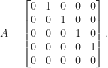
 , has two negative eigenvalues and a zero eigenvalue:
 . Is this the best choice?
 is minimized over symmetric
  for all unitary
  since
since  is optimal is simple. For any symmetric


 for symmetric
  . For the
 , and
, and  for any
  such that
  .
. is the nearest Hermitian matrix to
  is the nearest skew-Hermitian matrix to