A polar decomposition of  with
with  is a factorization
  , where
  has orthonormal columns and
  is Hermitian positive semidefinite. This decomposition is a generalization of the polar representation
  of a complex number, where
  corresponds to
  and
and  to
to  . When
  is real, is symmetric positive semidefinite. When
  , is a square unitary matrix (orthogonal for real ).
We have  , so
, so  , which is the unique positive semidefinite square root of
  . When has full rank, is nonsingular and
  is unique, and in this case can be expressed as
An example of a polar decomposition is
![A = \left[\begin{array}{@{}rr} 4 & 0\\ -5 & -3\\ 2 & 6 \end{array}\right] = \sqrt{2}\left[\begin{array}{@{}rr} \frac{1}{2} & -\frac{1}{6}\\[\smallskipamount] -\frac{1}{2} & -\frac{1}{6}\\[\smallskipamount] 0 & \frac{2}{3} \end{array}\right] \cdot \sqrt{2}\left[\begin{array}{@{\,}rr@{}} \frac{9}{2} & \frac{3}{2}\\[\smallskipamount] \frac{3}{2} & \frac{9}{2} \end{array}\right] \equiv UH.](https://s0.wp.com/latex.php?latex=A+%3D+%5Cleft%5B%5Cbegin%7Barray%7D%7B%40%7B%7Drr%7D+4+%26+0%5C%5C+-5+%26+-3%5C%5C+2+%26+6+%5Cend%7Barray%7D%5Cright%5D+++%3D+++%5Csqrt%7B2%7D%5Cleft%5B%5Cbegin%7Barray%7D%7B%40%7B%7Drr%7D+%5Cfrac%7B1%7D%7B2%7D+%26+-%5Cfrac%7B1%7D%7B6%7D%5C%5C%5B%5Csmallskipamount%5D+-%5Cfrac%7B1%7D%7B2%7D+%26+-%5Cfrac%7B1%7D%7B6%7D%5C%5C%5B%5Csmallskipamount%5D+0+%26+%5Cfrac%7B2%7D%7B3%7D+%5Cend%7Barray%7D%5Cright%5D+++%5Ccdot+++%5Csqrt%7B2%7D%5Cleft%5B%5Cbegin%7Barray%7D%7B%40%7B%5C%2C%7Drr%40%7B%7D%7D+%5Cfrac%7B9%7D%7B2%7D+%26+%5Cfrac%7B3%7D%7B2%7D%5C%5C%5B%5Csmallskipamount%5D+%5Cfrac%7B3%7D%7B2%7D+%26+%5Cfrac%7B9%7D%7B2%7D+%5Cend%7Barray%7D%5Cright%5D+++%5Cequiv+UH.+&bg=ffffff&fg=222222&s=0&c=20201002)
For an example with a rank-deficient matrix consider
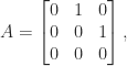
for which  and so
 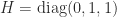 . The equation then implies that

so is not unique.
The polar factor has the important property that it is a closest matrix with orthonormal columns to in any unitarily invariant norm. Hence the polar decomposition provides an optimal way to orthogonalize a matrix. This method of orthogonalization is used in various applications, including in quantum chemistry, where it is called Löwdin orthogonalization. Most often, though, orthogonalization is done through QR factorization, trading optimality for a faster computation.
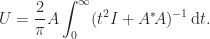
An important application of the polar decomposition is to the orthogonal Procrustes problem

where  and the norm is the Frobenius norm
  . This problem, which arises in factor analysis and in multidimensional scaling, asks how closely a unitary transformation of
  can reproduce . Any solution is a unitary polar factor of
  , and there is a unique solution if is nonsingular. Another application of the polar decomposition is in 3D graphics transformations. Here, the matrices are
  and the polar decomposition can be computed by exploiting a relationship with quaternions.
For a square nonsingular matrix , the unitary polar factor can be computed by a Newton iteration:

The iterates  converge quadratically to . This is just one of many iterations for computing and much work has been done on the efficient implementation of these iterations.
If  is a singular value decomposition (SVD), where
  has orthonormal columns,
  is unitary, and
  is square and diagonal with nonnegative diagonal elements, then

where has orthonormal columns and is Hermitian positive semidefinite. So a polar decomposition can be constructed from an SVD. The converse is true: if is a polar decomposition and  is a spectral decomposition (
 unitary,
  diagonal) then
 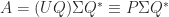 is an SVD. This latter relation is the basis of a method for computing the SVD that first computes the polar decomposition by a matrix iteration then computes the eigensystem of , and which is extremely fast on distributed-memory manycore computers.
The nonuniqueness of the polar decomposition for rank deficient , and the lack of a satisfactory definition of a polar decomposition for  , are overcome in the canonical polar decomposition, defined for any
  and
and  . Here, with a partial isometry, is Hermitian positive semidefinite, and
  . The superscript “
 ” denotes the Moore–Penrose pseudoinverse and a partial isometry can be characterized as a matrix for which
  .
.
Generalizations of the (canonical) polar decomposition have been investigated in which the properties of and are defined with respect to a general, possibly indefinite, scalar product.
References
This is a minimal set of references, which contain further useful references within.
- Nicholas J. Higham, Functions of Matrices: Theory and Computation, Society for Industrial and Applied Mathematics, Philadelphia, PA, USA, 2008. (Chapter 8.)
- Nicholas Higham, Christian Mehl, and Françoise Tisseur, The canonical generalized polar decomposition, SIAM J. Matrix Anal. Appl. 31(4), 2163–2180, 2010.
- Nicholas J. Higham and Vanni Noferini, An algorithm to compute the polar decomposition of a
 matrix, Numer. Algorithms 73, 349–369, 2016.
- Yuji Nakatsukasa and Nicholas J. Higham, Stable and efficient spectral divide and conquer algorithms for the symmetric eigenvalue decomposition and the SVD, SIAM J. Sci. Comput. 35(3), A1325–A1349, 2013.
- Dalal Sukkari, Hatem Ltaief, Aniello Esposito, and David Keyes, A QDWH-based SVD software framework on distributed-memory manycore systems, ACM Trans. Math. Software 45, 18:1–18:21, 2019.

I’m very much enjoying this “What is” series.
One question: At the beginning of this post you write: “This decomposition is a generalization of the polar representation z = r*e^(i*theta) of a complex number”. Can this analogy be taken further using the matrix exponential, setting U=e^V for some other matrix V?
Yes – there are standard results on writing an orthogonal or unitary matrix as exp(S) for a skew-symmetric or skew-Hermitian matrix.
You wrote, “Most often, though, orthogonalization is done through QR factorization, trading optimality for a faster computation.” One specific instance where QR decomposition is used is to generate Haar random unitary matrices. However, does the polar decomposition applied to an operator with independent and identically distributed Gaussian elements (i.i.d. Gaussian elements) also generate a Haar random unitary matrix?
You’re essentially asking whether $U = A(A^*A)^{-1/2}$ is Haar distributed for any Gaussian $A$. I haven’t seen a proof of that.