What Is a Pseudo-Orthogonal Matrix?

A matrix $Q\in\mathbb{R}^{n\times n}$ is pseudo-orthogonal if

$\notag Q^T \Sigma Q = \Sigma, \qquad (1)$

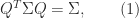
where $\Sigma = \mathrm{diag}(\pm 1)$ is a signature matrix. A matrix $Q$ satisfying (1) is also known as a $J$ -orthogonal matrix, where $J$ is another notation for a signature matrix. Of course, if $\Sigma = I$ then $Q$ is orthogonal.

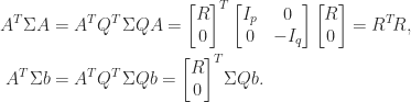
It is easy to show that $Q^T$ is also pseudo-orthogonal. Furthermore, $Q$ is clearly nonsingular and it satisfies

$\notag Q = \Sigma Q^{-T}\Sigma. \qquad (2)$

Since $\Sigma$ is orthogonal, this equation implies that $\|Q\|_\ell = \|Q^{-T}\|_\ell = \|Q^{-1}\|_\ell$ and hence that

$\notag \kappa_p(Q) = \|Q\|_\ell^2, \quad \ell = 2,F. \qquad(3).$

What are some examples of pseudo-orthogonal matrices? For $n = 2$ and $\Sigma = \left[\begin{smallmatrix}1 & 0 \\ 0 & -1 \end{smallmatrix}\right]$ , $Q$ is of the form

$\notag Q = \begin{bmatrix} a & b \\ c & d \end{bmatrix}, \quad ab - cd = 0, \quad a^2 - c^2 = 1, \quad b^2 - d^2 = -1,$

which includes the matrices

$\notag Q = \begin{bmatrix} \cosh \theta & -\sinh\theta \\ -\sinh\theta & \cosh\theta \end{bmatrix}, \quad \theta\in\mathbb{R}. \qquad (4)$

The Lorentz group, representing symmetries of the spacetime of special relativity, corresponds to $4\times 4$ matrices with $\Sigma = \mathrm{diag}(1,1,1,-1)$ .

Equation (2) shows that $Q$ is similar to the inverse of its transpose and hence (since every matrix is similar to its transpose) similar to its inverse. It follows that if $\lambda$ is an eigenvalue of $Q$ then $\lambda^{-1}$ is also an eigenvalue and it has the same algebraic and geometric multiplicities as $\lambda$ .

By permuting rows and columns in (1) we can arrange that

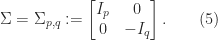
$\notag \Sigma = \Sigma_{p,q} := \begin{bmatrix} I_p & 0 \\ 0 & -I_q \end{bmatrix}. \qquad (5)$

We assume that $\Sigma$ has this form throughout the rest of this article. This form of $\Sigma$ allows us to conveniently characterize matrices that are both orthogonal and pseudo-orthogonal. Such a matrix must satisfy $\Sigma Q = Q\Sigma$ , which means that $Q = \mathrm{diag}(Q_{11},Q_{22})$ , and any such orthogonal matrix is pseudo-orthogonal.

Applications

Pseudo-orthogonal matrices arise in hyperbolic problems, that is, problems where there is an underlying indefinite scalar product or weight matrix. An example is the problem of downdating the Cholesky factorization, where in the simplest case we have the Cholesky factorization $C = R^T\!R$ of a symmetric positive definite $C\in\mathbb{R}^{n\times n}$ and want the Cholesky factorization of $\widetilde{C} = C - zz^T$ , which is assumed to be symmetric positive definite. A more general downdating problem is that we are given

$\notag A = \begin{array}[b]{cc} \left[\begin{array}{@{}c@{}} A_1\\ A_2 \end{array}\right] & \mskip-22mu\ \begin{array}{l} \scriptstyle p \\ \scriptstyle q \end{array} \end{array}, \quad p\ge n,$

and the Cholesky factorization $A^T\!A = R^T\!R$ and wish to obtain the Cholesky factor $S$ of $A_1^TA_1 = R^T\!R - A_2^TA_2$ . Note that $R$ and $S$ are $n\times n$ . This task arises when we solve a regression problem after the observations corresponding to $A_2$ have been removed. The simple case above corresponds to removing one row ( $q = 1$ ). Assuming that $q \ll p$ , we would like to obtain $S$ cheaply from $R$ , and numerical stability considerations dictate that we should avoid explicitly forming $A_1^TA_1$ . If we can find a pseudo-orthogonal matrix $Q$ such that

$\notag Q \begin{bmatrix} R \\ A_2 \end{bmatrix} = \begin{bmatrix} S \\ 0 \end{bmatrix}, \qquad (6)$

with $\Sigma$ given by (5) and $S\in\mathbb{R}^{n\times n}$ upper triangular, then

$\notag A_1^TA_1 = \begin{bmatrix} R \\ A_2 \end{bmatrix}^T \Sigma \begin{bmatrix} R \\ A_2 \end{bmatrix} = \begin{bmatrix} R \\ A_2 \end{bmatrix}^T Q^T \Sigma Q \begin{bmatrix} R \\ A_2 \end{bmatrix} = \begin{bmatrix} S \\ 0 \end{bmatrix}^T \Sigma \begin{bmatrix} S \\ 0 \end{bmatrix} = S^T\!S,$

so $S$ is the desired Cholesky factor.

The factorization (6) is called a hyperbolic QR factorization and it can be computed by using hyperbolic rotations to zero out the elements of $A_2$ . A $2\times2$ hyperbolic rotation has the form (4), and an $n\times n$ hyperbolic rotation is an identity matrix with a $2\times 2$ hyperbolic rotation embedded in it at the intersection of rows and columns $i$ and $j$ , for some $i$ and $j$ .

In general, a hyperbolic QR factorization of $A\in\mathbb{R}^{m\times n}$ with $m = p+q$ and $p\ge n$ has the form $QA = \left[\begin{smallmatrix} R \\ 0 \end{smallmatrix}\right]$ with $Q$ pseudo-orthogonal with respect to $\Sigma = \Sigma_{p,q}$ and $R \in\mathbb{R}^{n\times n}$ upper triangular. The factorization exists if $A^T\Sigma A$ is positive definite.

Another hyperbolic problem is the indefinite least squares problem

$\notag \min_x \,(b-Ax)^T \Sigma (b-Ax), \qquad (7)$

where $A\in\mathbb{R}^{m\times n}$ , $m\ge n$ , and $b\in\mathbb{R}^m$ are given, and $\Sigma = \Sigma_{p,q}$ with $m = p + q$ . For $p=0$ or $q=0$ we have the standard least squares (LS) problem and the quadratic form is definite, while for $pq>0$ the problem is to minimize a genuinely indefinite quadratic form. This problem arises, for example, in the area of optimization known as $H^{\infty}$ smoothing.

The normal equations for (7) are 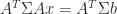$A^T\Sigma Ax = A^T\Sigma b$ , and since the Hessian matrix of the quadratic objective function in (7) is $A^T\Sigma A$ it follows that the indefinite least squares problem has a unique solution if and only if $A^T\Sigma A$ is positive definite. To solve the problem we can use a hyperbolic QR factorization $QA = \left[\begin{smallmatrix} R \\ 0 \end{smallmatrix}\right]$ to write

$\notag \begin{aligned} A^T\Sigma A &= A^T Q^T \Sigma Q A = \begin{bmatrix} R \\ 0 \end{bmatrix}^T \begin{bmatrix} I_p & 0 \\ 0 & -I_q \end{bmatrix} \begin{bmatrix} R \\ 0 \end{bmatrix} = R^T\!R, \\ A^T\Sigma b &= A^T Q^T\Sigma Q b = \begin{bmatrix} R \\ 0 \end{bmatrix}^T \! \Sigma Q b. \end{aligned}$

Solving the problem now reduces to solving the triangular system $Rx = d$ , where $d$ comprises the first $n$ components of $Qb$ . The same equation can also be obtained without using the normal equations by substituting the hyperbolic QR factorization into (7).

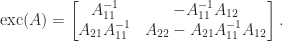
The Exchange Operator

A simple technique exists for converting pseudo-orthogonal matrices into orthogonal matrices and vice versa. Let $A\in\mathbb{R}^{n\times n}$ with $n = p + q$ , partition

$\notag A = \mskip5mu \begin{array}[b]{@{\mskip-20mu}c@{\mskip0mu}c@{\mskip-1mu}c@{}} & \mskip10mu\scriptstyle p & \scriptstyle q \\ \mskip15mu \begin{array}{r} \scriptstyle p \\ \scriptstyle q \end{array}~ & \multicolumn{2}{c}{\mskip-15mu \left[\begin{array}{c@{~}c@{~}} A_{11} & A_{12}\\ A_{21} & A_{22} \end{array}\right] } \end{array}, \qquad (8)$

and assume $A_{11}$ is nonsingular. The exchange operator is defined by

$\notag \mathrm{exc}(A) = \begin{bmatrix} A_{11}^{-1} & -A_{11}^{-1}A_{12} \\ A_{21}A_{11}^{-1} & A_{22} -A_{21}A_{11}^{-1}A_{12} \end{bmatrix}.$

It is easy to see that the exchange operator is involutory, that is,

$\notag \mathrm{exc}(\mathrm{exc}(A)) = A,$

and moreover (recalling that $\Sigma$ is given by (5)) that

$\notag \mathrm{exc}(\Sigma A\Sigma) = \Sigma \mathrm{exc}(A)\Sigma = \mathrm{exc}(A^T)^T. \qquad(9)$

The next result gives a formula for the inverse of $\mathrm{exc}(A)$ .

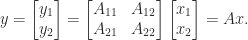
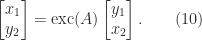
Lemma 1. Let $A\in\mathbb{R}^{n\times n}$ with $A_{11}$ nonsingular. If $A$ is nonsingular and $\mathrm{exc}(A^{-1})$ exists then $\mathrm{exc}(A)$ is nonsingular and $\mathrm{exc}(A)^{-1} = \mathrm{exc}(A^{-1})$ .

Proof. Consider the equation

$\notag y = \begin{bmatrix} y_1 \\ y_2 \end{bmatrix} = \begin{bmatrix} A_{11} & A_{12} \\ A_{21} & A_{22} \end{bmatrix} \begin{bmatrix} x_1 \\ x_2 \end{bmatrix} = Ax.$

By solving the first equation for $x_1$ and then eliminating $x_1$ from the second equation we obtain

$\notag \begin{bmatrix} x_1 \\ y_2 \end{bmatrix} = \mathrm{exc}(A) \begin{bmatrix} y_1 \\ x_2 \end{bmatrix}. \qquad (10)$

By the same argument applied to $x = A^{-1}y$ , we have

$\notag \begin{bmatrix} y_1 \\ x_2 \end{bmatrix} = \mathrm{exc}(A^{-1}) \begin{bmatrix} x_1 \\ y_2 \end{bmatrix}.$

Hence for any $x_1$ and $y_2$ there is a unique $y_1$ and $x_2$ , which implies by (10) that $\mathrm{exc}(A)$ is nonsingular and that $\mathrm{exc}(A)^{-1} = \mathrm{exc}(A^{-1})$ . $~\square$

Now we will show that the exchange operator maps pseudo-orthogonal matrices to orthogonal matrices and vice versa.

Theorem 2. Let $A\in\mathbb{R}^{n\times n}$ . If $A$ is pseudo-orthogonal then $\mathrm{exc}(A)$ is orthogonal. If $A$ is orthogonal and $A_{11}$ is nonsingular then $\mathrm{exc}(A)$ is pseudo-orthogonal.

Proof. If $A$ is pseudo-orthogonal then $A_{11}^TA_{11} = I + A_{21}^TA_{21}$ , which implies that $A_{11}$ is nonsingular. Since $\Sigma A^T\Sigma = A^{-1}$ , it follows that $A^{-1}$ also has a nonsingular $(1,1)$ block and so $\mathrm{exc}(A^{-1})$ exists. Furthermore, using Lemma 1, $\mathrm{exc}(\Sigma A^T\Sigma) = \mathrm{exc}(A^{-1}) = \mathrm{exc}(A)^{-1}$ . But (9) shows that $\mathrm{exc}(\Sigma A^T\Sigma) = \mathrm{exc}(A)^T$ , and we conclude that $\mathrm{exc}(A)$ is orthogonal.

Assume now that $A$ is orthogonal with $A_{11}$ nonsingular. Then $\mathrm{exc}(A^T) = \mathrm{exc}(A^{-1})$ exists and Lemma 1 shows that $\mathrm{exc}(A)$ is nonsingular and $\mathrm{exc}(A)^{-1} = \mathrm{exc}(A^{-1}) = \mathrm{exc}(A^T)$ . Hence, using (9),

$I = \mathrm{exc}(A^T) \mathrm{exc}(A) = \Sigma\mathrm{exc}(A)^T\Sigma \cdot \mathrm{exc}(A),$

which shows that $\mathrm{exc}(A)$ is pseudo-orthogonal. $~\square$

This MATLAB example uses the exchange operator to convert an orthogonal matrix obtained from a Hadamard matrix into a pseudo-orthogonal matrix.

>> p = 2; n = 4;
>> A = hadamard(n)/sqrt(n), Sigma = blkdiag(eye(p),-eye(n-p))
A =
   5.0000e-01   5.0000e-01   5.0000e-01   5.0000e-01
   5.0000e-01  -5.0000e-01   5.0000e-01  -5.0000e-01
   5.0000e-01   5.0000e-01  -5.0000e-01  -5.0000e-01
   5.0000e-01  -5.0000e-01  -5.0000e-01   5.0000e-01
Sigma =
     1     0     0     0
     0     1     0     0
     0     0    -1     0
     0     0     0    -1
>> Q = exc(A,p), Q'*Sigma*Q
Q =
     1     1    -1     0
     1    -1     0    -1
     1     0    -1    -1
     0     1    -1     1
ans =
     1     0     0     0
     0     1     0     0
     0     0    -1     0
     0     0     0    -1

The code uses the function

function X = exc(A,p)
%EXC     Exchange operator.
%   EXC(A,p) is the result of applying the exchange operator to 
%   the square matrix A, which is regarded as a block 2-by-2 
%   matrix with leading block of dimension p.  
%   p defaults to floor(n)/2.

[m,n] = size(A);
if m ~= n, error('Matrix must be square.'), end
if nargin < 2, p = floor(n/2); end

A11 = A(1:p,1:p);
A12 = A(1:p,p+1:n);
A21 = A(p+1:n,1:p);
A22 = A(p+1:n,p+1:n);

X21 = A11\A12;
X = [inv(A11) -X21;
     A21/A11  A22-A21*X21];

Hyperbolic CS Decomposition

For an orthogonal matrix expressed in block $2\times 2$ form there is a close relationship between the singular value decompositions (SVDs) of the blocks, as revealed by the CS decomposition (see What Is the CS Decomposition?). An analogous decomposition holds for a pseudo-orthogonal matrix. Let $Q\in\mathbb{R}^{n \times n}$ be pseudo-orthogonal with respect to $\Sigma$ in (5), and suppose that $Q$ is partitioned as

$\notag Q = \begin{array}[b]{@{\mskip33mu}c@{\mskip-16mu}c@{\mskip-10mu}c@{}} \scriptstyle p & \scriptstyle n-p & \\ \multicolumn{2}{c}{ \left[\begin{array}{c@{~}c@{~}} Q_{11}& Q_{12} \\ Q_{21}& Q_{22} \\ \end{array}\right]} & \mskip-12mu\ \begin{array}{c} \scriptstyle p \\ \scriptstyle n-p \end{array} \end{array}, \quad p \le \displaystyle\frac{n}{2}.$

Then there exist orthogonal matrices $U_1,V_1\in\mathbb{R}^{p \times p}$ and $U_2,V_2\in\mathbb{R}^{q \times q}$ such that

$\notag \begin{bmatrix} U_1^T & 0\\ 0 & U_2^T \end{bmatrix} \begin{bmatrix} Q_{11} & Q_{12}\\ Q_{21} & Q_{22} \end{bmatrix} \begin{bmatrix} V_1 & 0\\ 0 & V_2 \end{bmatrix} = \begin{array}[b]{@{\mskip35mu}c@{\mskip30mu}c@{\mskip-10mu}c@{}c} \scriptstyle p & \scriptstyle p & \scriptstyle n-2p & \\ \multicolumn{3}{c}{ \left[\begin{array}{c@{~}|c@{~}c} C & -S & 0 \\ \hline -S & C & 0 \\ 0 & 0 & I_{n-2p} \end{array}\right]} & \mskip-12mu \begin{array}{c} \scriptstyle p \\ \scriptstyle p \\ \scriptstyle n-2p \end{array} \end{array}, \qquad (11)$

where $C = \mathrm{diag}(c_i)$ , $S = \mathrm{diag}(s_i)$ , and $C^2 - S^2 = I$ , with $c_i > s_i \ge 0$ for all $i$ . This is the hyperbolic CS decomposition, and it can be proved by applying the CS decomposition of an orthogonal matrix to $\mathrm{exc}(Q)$ .

The leading principal submatrix $\left[\begin{smallmatrix}C & -S \\ -S & C \end{smallmatrix}\right]$ in (11) generalizes the $2\times 2$ matrix (4), and in fact it can be permuted into a direct sum of such matrices.

Note that the matrix on the right in (11) is symmetric positive definite. Therefore the singular values of $Q$ are the eigenvalues of that matrix, namely

$\notag c_1 \pm s_1, \dots, c_p \pm s_p; \quad 1~\mathrm{with~multiplicity~}n - 2p.$

Since $c_i^2 - s_i^2 = 1$ for all $i$ , the first $2p$ singular values occur in reciprocal pairs, hence the largest and smallest singular values satisfy $\sigma_1 = \sigma_n^{-1}\ge 1$ (with strict inequality unless $p = 0$ ). This gives another proof of (3).

Numerical Stability

While an orthogonal matrix is perfectly conditioned, a pseudo-orthogonal matrix can be arbitrarily ill conditioned, as follows from (3). For example, the MATLAB function gallery('randjorth') produces a random pseudo-orthogonal matrix with a default condition number of sqrt(1/eps).

>> rng(1); A = gallery('randjorth',2,2) % p = 2, n = 4
A =
   2.9984e+03  -4.2059e+02   1.5672e+03  -2.5907e+03
   1.9341e+03  -2.6055e+03   3.1565e+03  -7.5210e+02
   3.1441e+03  -6.2852e+02   1.8157e+03  -2.6427e+03
   1.6870e+03  -2.5633e+03   3.0204e+03  -5.4157e+02
>> cond(A)
ans =
   6.7109e+07

This means that algorithms that use pseudo-orthogonal matrices are potentially numerically unstable. Therefore algorithms need to be carefully constructed and rounding error analysis must be done to ensure that an appropriate form of numerical stability is obtained.

Notes

Pseudo-orthogonal matrices form the automorphism group of the scalar product defined by $\langle x,y\rangle = x^T\Sigma y$ for $x,y\in\mathbb{R}^n$ . More results for pseudo-orthogonal matrices can be obtained as special cases of results for automorphism groups of general scalar products. See, for example, Mackey, Mackey, and Tisseur (2006).

For $\Sigma \ne \pm I$ the set of pseudo-orthogonal matrices is known to have four connected components, a topological property that can be proved using the hyperbolic CS decomposition (Motlaghian, Armandnejad, and Hall, 2018).

One can define pseudo-unitary matrices in an analogous way, as $Q\in\mathbb{C}^{n\times n}$ such that $Q^*\Sigma Q = \Sigma$ . These correspond to the automorphism group of the scalar product $\langle x,y\rangle = x^*\Sigma y$ for $x,y\in\mathbb{C}^n$ . The results we have discussed generalize in a straightforward way to pseudo-unitary matrices.

The exchange operator is also known as the principal pivot transform and as the sweep operator in statistics. Tsatsomeros (2000) gives a survey of its properties

The hyperbolic CS decomposition was derived by Lee (1948) and, according to Lee, was present in work of Autonne (1912).

References

This is a minimal set of references, which contain further useful references within.

Adam Bojanczyk, Nicholas J. Higham and Harikrishna Patel, Solving the Indefinite Least Squares Problem by Hyperbolic QR Factorization, SIAM J. Matrix Anal. Appl. 24(3), 914–931, 2003
Nicholas J. Higham, $J$ -Orthogonal Matrices: Properties and Generation, SIAM Rev. 45(3), 504–519, 2003
H. C. Lee, Canonical Factorization of Pseudo-Unitary Matrices, Proc. London Math. Soc. s2-50, 230–241, 1948.
D. Steven Mackey, Niloufer Mackey, and Françoise Tisseur, Structured Factorizations in Scalar Product Spaces, SIAM J. Matrix Anal. Appl. 27(3), 821–850, 2006.
Sara M. Motlaghian, Ali Armandnejad, and Frank J. Hall, Topological Properties of $J$ -Orthogonal Matrices, Linear and Multilinear Algebra 66(12), 2524–2533, 2018.
Michael Stewart and G. W. Stewart, On Hyperbolic Triangularization: Stability and Pivoting, SIAM J. Matrix Anal. Appl. 19(4), 847–860, 1998
Michael J. Tsatsomeros, Principal Pivot Transforms: Properties and Applications, Linear Algebra Appl. 307, 151–165, 2000.

What Is a Pseudo-Orthogonal Matrix?

Applications

The Exchange Operator

Hyperbolic CS Decomposition

Numerical Stability

Notes

References

Related Blog Posts

Leave a comment Cancel reply

Applications

The Exchange Operator

Hyperbolic CS Decomposition

Numerical Stability

Notes

References

Related Blog Posts

Share this:

Related

Leave a comment Cancel reply