A companion matrix 

Alternatively, 


so the coefficients in the first row of 


Setting 


Note that 


A companion matrix has some low rank structure. It can be expressed as a unitary matrix plus a rank-

Also, 


If 
![[\lambda^{n-1}, \lambda^{n-2}, \dots, \lambda, 1]^T](https://s0.wp.com/latex.php?latex=%5B%5Clambda%5E%7Bn-1%7D%2C+%5Clambda%5E%7Bn-2%7D%2C+%5Cdots%2C+%5Clambda%2C+1%5D%5ET&bg=ffffff&fg=222222&s=0&c=20201002)

The MATLAB function compan takes as input a vector ![[p_1,p_2, \dots, p_{n+1}]](https://s0.wp.com/latex.php?latex=%5Bp_1%2Cp_2%2C+%5Cdots%2C+p_%7Bn%2B1%7D%5D&bg=ffffff&fg=222222&s=0&c=20201002)


Perhaps surprisingly, the singular values of

where 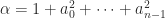
Applications
Companion matrices arise naturally when we convert a high order difference equation or differential equation to first order. For example, consider the Fibonacci numbers 


where ![\left[\begin{smallmatrix}1 & 1 \\ 1 & 0 \end{smallmatrix}\right]](https://s0.wp.com/latex.php?latex=%5Cleft%5B%5Cbegin%7Bsmallmatrix%7D1+%26+1+%5C%5C+1+%26+0+%5Cend%7Bsmallmatrix%7D%5Cright%5D&bg=ffffff&fg=222222&s=0&c=20201002)


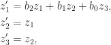
As another example, consider the differential equation
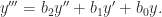
Define new variables

Then
or

so the third order scalar equation has been converted into a first order system with a companion matrix as coefficient matrix.
Computing Polynomial Roots
The MATLAB function roots takes as input a vector of the coefficients of a polynomial and returns the roots of the polynomial. It computes the eigenvalues of the companion matrix associated with the polynomial using the eig function. As Moler (1991) explained, MATLAB used this approach starting from the first version of MATLAB, but it does not take advantage of the structure of the companion matrix, requiring 


Rational Canonical Form
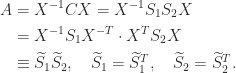
It is an interesting observation that

Multiplying by the inverse of the matrix on the left we express the 


We need the rational canonical form of a matrix, described in the next theorem, which Halmos (1991) calls “the deepest theorem of linear algebra”. Let 


Theorem 1 (rational canonical form).
If
then
where
is nonsingular and
, with each
a companion matrix.
The theorem says that every matrix is similar over the underlying field to a block diagonal matrix composed of companion matrices. Since we do not need it, we have omitted from the statement of the theorem the description of the
Since 


Theorem 2 (Frobenius, 1910).
For any
, either one of which can be taken nonsingular, such that
.
Note that if 


Factorization
Fiedler (2003) noted that a companion matrix can be factorized into the product of 


![\notag \widetilde{C} = \begin{bmatrix} a_4 & a_3 & 1 & 0 & 0 \\ 1 & 0 & 0 & 0 & 0 \\ 0 & a_2 & 0 & a_1 & 1 \\ 0 & 1 & 0 & 0 & 0 \\ 0 & 0 & 0 & a_0 & 0 \end{bmatrix} = \left[\begin{array}{cc|cc|c} a_4 & 1 & & & \\ 1 & 0 & & & \\\hline & & a_2 & 1 & \\ & & 1 & 0 & \\\hline & & & & a_0 \end{array}\right] \left[\begin{array}{c|cc|cc} 1 & & & & \\\hline & a_3 & 1 & & \\ & 1 & 0 & & \\\hline & & & a_1 & 1 \\ & & & 1 & 0 \end{array}\right].](https://s0.wp.com/latex.php?latex=%5Cnotag+%5Cwidetilde%7BC%7D+%3D+%5Cbegin%7Bbmatrix%7D++++a_4+%26+a_3+%26+1++%26+0+++%26+0++%5C%5C++++++1+%26+0+++%26+0++%26+0+++%26+0++%5C%5C++++++0+%26+a_2+%26+0++%26+a_1+%26+1++%5C%5C++++++0+%26+1+++%26+0++%26+0+++%26+0+%5C%5C++++++0+%26+0+++%26+0++%26+a_0+%26+0+%5Cend%7Bbmatrix%7D+%3D+%5Cleft%5B%5Cbegin%7Barray%7D%7Bcc%7Ccc%7Cc%7D++++a_4+%26+1+%26+++++%26+++%26+++%5C%5C++++++1+%26+0+%26+++++%26+++%26+++%5C%5C%5Chline++++++++%26+++%26+a_2+%26+1+%26+++%5C%5C++++++++%26+++%26++1++%26+0+%26+++%5C%5C%5Chline++++++++%26+++%26+++++%26+++%26++a_0+%5Cend%7Barray%7D%5Cright%5D+%5Cleft%5B%5Cbegin%7Barray%7D%7Bc%7Ccc%7Ccc%7D++++++1++%26+++++%26+++%26++++++%26+%5C%5C%5Chline+++++++++%26+a_3+%26+1+%26++++++%26+%5C%5C+++++++++%26++1++%26+0+%26++++++%26+%5C%5C%5Chline+++++++++%26+++++%26+++%26++a_1+%26+1+%5C%5C+++++++++%26+++++%26+++%26+++1++%26+0+%5Cend%7Barray%7D%5Cright%5D.+&bg=ffffff&fg=222222&s=0&c=20201002)
In general, Fielder’s construction yields an
Generalizations
The companion matrix is associated with the monomial basis representation of the characteristic polynomial. Other polynomial bases can be used, notably orthogonal polynomials, and this leads to generalizations of the companion matrix having coefficients on the main diagonal and the subdiagonal and superdiagonal. Good (1961) calls the matrix resulting from the Chebyshev basis a colleague matrix. Barnett (1981) calls the matrices corresponding to orthogonal polynomials comrade matrices, and for a general polynomial basis he uses the term confederate matrices. Generalizations of the properties of companion matrices can be derived for these classes of matrices.
Bounds for Polynomial Roots
Since the roots of a polynomial are the eigenvalues of the associated companion matrix, or a Fiedler matrix similar to it, or indeed the associated comrade matrix or confederate matrix, one can obtain bounds on the roots by applying any available bounds for matrix eigenvalues. For example, since any eigenvalue 


either of which can be the smaller. A rich variety of such bounds is available, and these techniques extend to matrix polynomials and the corresponding block companion matrices.
References
This is a minimal set of references, which contain further useful references within.
- Jared L. Aurentz, Thomas Mach, Raf Vandebril, and David S. Watkins, Fast and Backward Stable Computation of Roots of Polynomials, SIAM J. Matrix Anal. Appl. 36(3), 942–973, 2015.
- Stephen Barnett, Congenial Matrices, Linear Algebra Appl. 41, 277–298, 1981.
- Fernando De Terán and Froilán M. Dopico and Javier Pérez, New Bounds for Roots of Polynomials Based on Fiedler Companion Matrices, Linear Algebra Appl. 451, 197–230, 2014.
- Miroslav Fiedler, A Note on Companion Matrices, Linear Algebra Appl. 372, 325–331, 2003.
- Nicholas J. Higham and Françoise Tisseur, Bounds for Eigenvalues of Matrix Polynomials, Linear Algebra Appl. 358, 5–22, 2003
- Charles S. Kenney and Alan J. Laub, Controllability and Stability Radii for Companion Form Systems, Math. Control Signals Systems 1, 239–256, 1988.
- Cyrus Colton MacDuffee, The Theory of Matrices, Chelsea, New York, 1946.
- D. Steven Mackey, The Continuing Influence of Fiedler’s Work on Companion Matrices, Linear Algebra Appl. 439, 810–817, 2013.
- Cleve Moler, ROOTS—of Polynomials, That Is, The MathWorks Newsletter 5(1), 1991.
- Olga Taussky, The Role of Symmetric Matrices in the Study of General Matrices, Linear Algebra Appl. 5, 147–154, 1972.
Related Blog Posts
This article is part of the “What Is” series, available from https://nhigham.com/category/what-is and in PDF form from the GitHub repository https://github.com/higham/what-is.
