An 


The definition says that the inner product of the 


For a general diagonalizable matrix, 


Many equivalent conditions to
The normal matrices include the classes of matrix given in this table:
| Real | Complex |
|---|---|
| Diagonal | Diagonal |
| Symmetric | Hermitian |
| Skew-symmetric | Skew-Hermitian |
| Orthogonal | Unitary |
| Circulant | Circulant |
Circulant matrices are
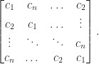
They are diagonalized by a unitary matrix known as the discrete Fourier transform matrix, which has 

A normal matrix is not necessarily of the form given in the table, even for 

![\notag \left[\begin{array}{@{\mskip2mu}rr@{\mskip2mu}} a & b\\ b & c \end{array}\right], \quad \left[\begin{array}{@{}rr@{\mskip2mu}} a & b\\ -b & a \end{array}\right].](https://s0.wp.com/latex.php?latex=%5Cnotag++++%5Cleft%5B%5Cbegin%7Barray%7D%7B%40%7B%5Cmskip2mu%7Drr%40%7B%5Cmskip2mu%7D%7D++++++a+%26+b%5C%5C++++++b+%26+c++++%5Cend%7Barray%7D%5Cright%5D%2C+%5Cquad++++%5Cleft%5B%5Cbegin%7Barray%7D%7B%40%7B%7Drr%40%7B%5Cmskip2mu%7D%7D++++++a+%26+b%5C%5C+++++-b+%26+a++++%5Cend%7Barray%7D%5Cright%5D.+&bg=ffffff&fg=222222&s=0&c=20201002)
The first matrix is symmetric. The second matrix is of the form 
![J = \bigl[\begin{smallmatrix}\!\phantom{-}0 & 1\\\!-1 & 0 \end{smallmatrix}\bigr]](https://s0.wp.com/latex.php?latex=J+%3D+%5Cbigl%5B%5Cbegin%7Bsmallmatrix%7D%5C%21%5Cphantom%7B-%7D0+%26+1%5C%5C%5C%21-1+%26+0+%5Cend%7Bsmallmatrix%7D%5Cbigr%5D&bg=ffffff&fg=222222&s=0&c=20201002)


It is natural to ask what the commutator 

In the polar decomposition 


The field of values, also known as the numerical range, is defined for 
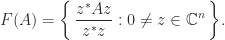
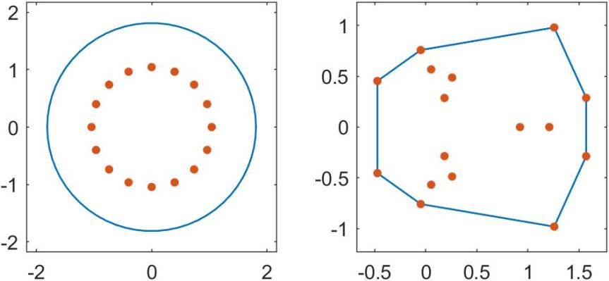
The set 
gallery('smoke',16) and that on the right is for the circulant matrix gallery('circul',x) with x constructed as x = randn(16,1); x = x/norm(x).
Measures of Nonnormality
How can we measure the degree of nonnormality of a matrix? Let 


Henrici (1962) derived an upper bound for 
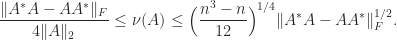
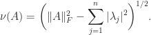
The distance to normality is

This quantity can be computed by an algorithm of Ruhe (1987). It is trivially bounded above by
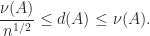
Normal matrices are a particular class of diagonalizable matrices. For diagonalizable matrices various bounds are available that depend on the condition number of a diagonalizing transformation. Since such a transformation is not unique, we take a diagonalization

Here are some examples of such bounds. We denote by 
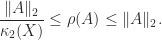
- By taking norms in the eigenvalue-eigenvector equation
we obtain
. Taking norms in
. Hence
- If
and its eigenvalues are ordered
, then (Ruhe, 1975)
Note that for
the previous upper bound is sharper.
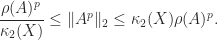
- For any real
,
- For any function
defined on the spectrum of

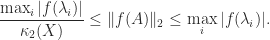
For normal 
References
This is a minimal set of references, which contain further useful references within.
- L. Elsner and Kh.D. Ikramov, Normal Matrices: An Update, Linear Algebra Appl 285, 291–303, 1998.
- L. Elsner and M. H. C. Paardekooper, On Measures of Nonnormality of Matrices, Linear Algebra Appl. 92, 107–124, 1987.
- Robert Grone, Charles Johnson, Eduardo Sa, and Henry Wolkowicz, Normal Matrices, Linear Algebra Appl. 87, 213–225, 1987
- Peter Henrici, Bounds for Iterates, Inverses, Spectral Variation and Fields of Values of Non-Normal Matrices, Numer. Math. 4, 24–40, 1962.
- Lajos László, An Attainable Lower Bound for the Best Normal Approximation, SIAM J. Matrix Anal. Appl. 15 (3), 1035–1043, 1994.
- Axel Ruhe, On the Closeness of Eigenvalues and Singular Values Of Almost Normal Matrices, Linear Algebra Appl. 11, 87–94, 1975.
- Axel Ruhe, Closest Normal Matrix Finally Found!, BIT 27, 585–598, 1987.
