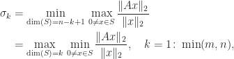
We present a selection of bounds for the condition number 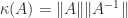

General Matrices
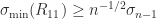
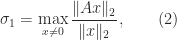
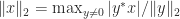
From the inequality 


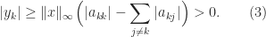
Fir the 

Guggenheimer, Edelman, and Johnson (1995) obtain the bound

The proof of the bound applies the arithmetic–geometric mean inequality to the 


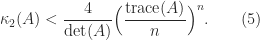
Merikoski, Urpala, Virtanen, Tam, and Uhlig (1997) obtain the bound

Their proof uses a more refined application of the arithmetic–geometric mean inequality, and they show that this bound is the smallest that can be obtained based on 


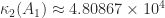
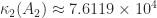
As an example, for three random 

gallery('randsvd') with three different singular value dsitributions:
| Mode | (2) | (3) |
|---|---|---|
| One large singular value | 9.88e+07 | 9.88e+07 |
| One small singular value | 1.21e+01 | 1.20e+01 |
| Geometrically distributed singular values | 5.71e+04 | 5.71e+04 |
We note that for larger 
Hermitian Positive Definite Matrices
Merikoski et al. (1997) also give a version of (3) for Hermitian positive definite

This is the smallest bound that can be obtained based on 


which gives the weaker bound
This bound is analogous to (2) and is up to a factor 

If 

These bounds hold for any positive definite matrix with unit diagonal, that is, any nonsingular correlation matrix.
We can sometimes get a sharper bound than (4) and (5) by writing 


and bounding 

![\notag P_5 = \left[\begin{array}{ccccc} 1 & 1 & 1 & 1 & 1\\ 1 & 2 & 3 & 4 & 5\\ 1 & 3 & 6 & 10 & 15\\ 1 & 4 & 10 & 20 & 35\\ 1 & 5 & 15 & 35 & 70 \end{array}\right]](https://s0.wp.com/latex.php?latex=%5Cnotag+P_5+%3D+%5Cleft%5B%5Cbegin%7Barray%7D%7Bccccc%7D+1+%26+1+%26+1+%26+1+%26+1%5C%5C+1+%26+2+%26+3+%26+4+%26+5%5C%5C+1+%26+3+%26+6+%26+10+%26+15%5C%5C+1+%26+4+%26+10+%26+20+%26+35%5C%5C+1+%26+5+%26+15+%26+35+%26+70+%5Cend%7Barray%7D%5Cright%5D+&bg=ffffff&fg=222222&s=0&c=20201002)
the condition number is 


Notes
Many other condition number bounds are available in the literature. All have their pros and cons and any bound based on limited information such as traces of powers of
A drawback of the bounds (3)–(6) is that they require 

The bounds (3) and (4) are used by Higham and Lettington (2021) in investigating the most ill conditioned 

References
This is a minimal set of references, which contain further useful references within.
- Heinrich Guggenheimer, Alan Edelman, and Charles Johnson, A Simple Estimate of the Condition Number of a Linear System, College Math. J. 26, 2–5, 1995.
- Nicholas J. Higham, Accuracy and Stability of Numerical Algorithms, second edition, Society for Industrial and Applied Mathematics, Philadelphia, PA, USA, 2002.
- Nicholas J. Higham and Matthew C. Lettington, Optimizing and Factorizing the Wilson Matrix, to appear in Amer. Math. Monthly, 2021.
- Jorma Kaarlo Merikoski, Uoti Urpala, Ari Virtanen, Tin-Yau Tam, and Frank Uhlig, A Best Upper Bound for the 2-Norm Condition Number of a Matrix, Linear Algebra Appl. 254, 355–365, 1997.
 and inverse
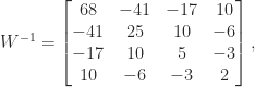
 . This little matrix has been used as an example and for test purposes in many research papers and books over the years, in particular by John Todd, who described it as “the notorious matrix
  of T. S. Wilson”.
 for a “positive definite symmetric
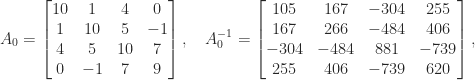
 . The matrix
  is therefore a factor 12 more ill conditioned than
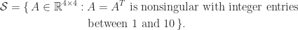
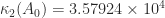
 and found that about 0.21 percent of them had a larger condition number than
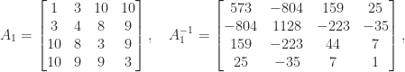
 . How far is this matrix from being a worst case?
 . It is possible to obtain a bound from first principles by using the relation
  , where
  is the
  ,
,
 , using the fact that
  is monotonically increasing for
  , gives
 ,
,
 , since
  we have
  , and hence
 . The bounds (1) and (2) remain valid if we modify the definitions of
  to allow zero elements (note that Rutishauser’s matrix
  elements. Exhaustively searching over the sets in reasonable time is possible with a carefully optimized code. Higham and Lettington (2021) use a MATLAB code that loops over all symmetric matrices with integer elements between
  of
of  (since
 . and determinant
  . The maximum over
 and determinant


![\notag R = \begin{bmatrix} \sqrt{5} & \frac{7\,\sqrt{5}}{5} & \frac{6\,\sqrt{5}}{5} & \sqrt{5}\\[\smallskipamount] 0 & \frac{\sqrt{5}}{5} & -\frac{2\,\sqrt{5}}{5} & 0\\[\smallskipamount] 0 & 0 & \sqrt{2} & \frac{3\,\sqrt{2}}{2}\\[\smallskipamount] 0 & 0 & 0 & \frac{\sqrt{2}}{2} \end{bmatrix} \quad (W = R^TR).](https://s0.wp.com/latex.php?latex=%5Cnotag+R+%3D+%5Cbegin%7Bbmatrix%7D+%5Csqrt%7B5%7D+%26+%5Cfrac%7B7%5C%2C%5Csqrt%7B5%7D%7D%7B5%7D+%26+%5Cfrac%7B6%5C%2C%5Csqrt%7B5%7D%7D%7B5%7D+%26+%5Csqrt%7B5%7D%5C%5C%5B%5Csmallskipamount%5D+0+%26+%5Cfrac%7B%5Csqrt%7B5%7D%7D%7B5%7D+%26+-%5Cfrac%7B2%5C%2C%5Csqrt%7B5%7D%7D%7B5%7D+%26+0%5C%5C%5B%5Csmallskipamount%5D+0+%26+0+%26+%5Csqrt%7B2%7D+%26+%5Cfrac%7B3%5C%2C%5Csqrt%7B2%7D%7D%7B2%7D%5C%5C%5B%5Csmallskipamount%5D+0+%26+0+%26+0+%26+%5Cfrac%7B%5Csqrt%7B2%7D%7D%7B2%7D+%5Cend%7Bbmatrix%7D+%5Cquad+%28W+%3D+R%5ETR%29.+&bg=ffffff&fg=222222&s=0&c=20201002)
 element, it is unremarkable. If we factor out the diagonal then we obtain the
  factorization, which has rational elements:
 with a
  matrix
  of integers. It is known that every symmetric positive definite
  matrix
  with
with  , but examples are known for
  for which the factorization does not exist. This result is mentioned by Taussky (1961) and goes back to Hermite, Minkowski, and Mordell. Higham and Lettington (2021) found the integer factor
 it is necessary that a certain quadratic equation in
 and two rational factors:
![\notag Z_1=\left[ \begin{array}{cccc} \frac{1}{2} & 1 & 0 & 1 \\ \frac{3}{2} & 2 & 3 & 3 \\ \frac{1}{2} & 1 & 0 & 0 \\ \frac{3}{2} & 2 & 1 & 0 \\ \end{array} \right], \quad Z_2=\left[ \begin{array}{@{\mskip2mu}rrrr} \frac{3}{2} & 2 & 2 & 2 \\ \frac{3}{2} & 2 & 2 & 1 \\ \frac{1}{2} & 1 & 1 & 2 \\ -\frac{1}{2} & -1 & 1 & 1 \\ \end{array} \right].](https://s0.wp.com/latex.php?latex=%5Cnotag+Z_1%3D%5Cleft%5B+%5Cbegin%7Barray%7D%7Bcccc%7D++%5Cfrac%7B1%7D%7B2%7D+%26+1+%26+0+%26+1+%5C%5C++%5Cfrac%7B3%7D%7B2%7D+%26+2+%26+3+%26+3+%5C%5C++%5Cfrac%7B1%7D%7B2%7D+%26+1+%26+0+%26+0+%5C%5C++%5Cfrac%7B3%7D%7B2%7D+%26+2+%26+1+%26+0+%5C%5C+%5Cend%7Barray%7D+%5Cright%5D%2C+%5Cquad+Z_2%3D%5Cleft%5B+%5Cbegin%7Barray%7D%7B%40%7B%5Cmskip2mu%7Drrrr%7D++%5Cfrac%7B3%7D%7B2%7D+%26+2+%26+2+%26+2+%5C%5C++%5Cfrac%7B3%7D%7B2%7D+%26+2+%26+2+%26+1+%5C%5C++%5Cfrac%7B1%7D%7B2%7D+%26+1+%26+1+%26+2+%5C%5C++-%5Cfrac%7B1%7D%7B2%7D+%26+-1+%26+1+%26+1+%5C%5C+%5Cend%7Barray%7D+%5Cright%5D.+&bg=ffffff&fg=222222&s=0&c=20201002)
 of
of  (a problem also considered in Higham, Lettington, and Schmidt (2021)), with integer
  has less than full rank, that is,
  . Sometimes,
  is known, and a full-rank factorization
  with
with  and
and  , both of rank
  or
or  . Often, though, the rank
 ,
,  , and
, and  and
and  are orthogonal. The Eckart–Young theorem says that
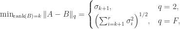

 is the best rank-
 approximation to
 ,
,  is diagonal and nonsingular, and
  and
and  are well conditioned.
 . Hence as long as
 for any permutation matrix
  and the second expression is another RRF). For
  we have
 from the rank-
 , which is the same order as the distance to the nearest rank-
 .
.  the numerical rank of
  .
.  with
with  . For the numerical rank to be meaningful in the sense that it is unchanged if
  is perturbed slightly, we need
  or
or  , which means that there must be a significant gap between these two singular values.
  , where
  has orthonormal columns,
  is upper triangular, and we assume that
  . In Definition 1, we can take
 ), and the prescription
  gives
gives  , so
, so  . The essential problem is that the diagonal of
  has no connection with the nonzero singular values of
  for the permutation matrix
  that reorders
 ![[a_1,a_2,a_3,a_4]](https://s0.wp.com/latex.php?latex=%5Ba_1%2Ca_2%2Ca_3%2Ca_4%5D&bg=ffffff&fg=222222&s=0&c=20201002) to
to ![[a_2,a_3,a_4,a_1]](https://s0.wp.com/latex.php?latex=%5Ba_2%2Ca_3%2Ca_4%2Ca_1%5D&bg=ffffff&fg=222222&s=0&c=20201002) , and this is a perfect RRF with
, and this is a perfect RRF with  .
. ![\notag A = \left[\begin{array}{rrrr} 1 & 1 &\theta &0\\ 1 & -1 & 2 &1 \\ 1 & 0 &1+\theta &-1\\ 1 &-1 & 2 &-1 \end{array}\right], \quad \theta = 10^{-8}. \qquad (\dagger)](https://s0.wp.com/latex.php?latex=%5Cnotag+++A+%3D+%5Cleft%5B%5Cbegin%7Barray%7D%7Brrrr%7D++++++++1+%26+1++%26%5Ctheta+%260%5C%5C++++++++1+%26+-1+%26+2+%261+%5C%5C++++++++1+%26+0++%261%2B%5Ctheta+%26-1%5C%5C++++++++1+%26-1++%26+2+%26-1+++%5Cend%7Barray%7D%5Cright%5D%2C+%5Cquad+%5Ctheta+%3D+10%5E%7B-8%7D.+%5Cqquad+%28%5Cdagger%29+&bg=ffffff&fg=222222&s=0&c=20201002)
 element tells us that
  of being rank deficient and so has a singular value bounded above by this quantity, but it does not provide any information about the next larger singular value. Moreover, in
  is of order
  for this factorization. We need any small diagonal elements to be in the bottom right-hand corner, and to achieve this we need to introduce column permutations to move the “dependent columns” to the end.
  , where

 with
with ![\notag R = \begin{array}[b]{@{\mskip33mu}c@{\mskip-16mu}c@{\mskip-10mu}c@{}} \scriptstyle k & \scriptstyle n-k & \\ \multicolumn{2}{c}{ \left[\begin{array}{c@{~}c@{~}} R_{11}& R_{12} \\ 0 & R_{22} \\ \end{array}\right]} & \mskip-12mu\ \begin{array}{c} \scriptstyle k \\ \scriptstyle n-k \end{array} \end{array}, \qquad(4)](https://s0.wp.com/latex.php?latex=%5Cnotag++++R+%3D++++%5Cbegin%7Barray%7D%5Bb%5D%7B%40%7B%5Cmskip33mu%7Dc%40%7B%5Cmskip-16mu%7Dc%40%7B%5Cmskip-10mu%7Dc%40%7B%7D%7D++++%5Cscriptstyle+k+%26++++%5Cscriptstyle+n-k+%26++++%5C%5C++++%5Cmulticolumn%7B2%7D%7Bc%7D%7B++++++++%5Cleft%5B%5Cbegin%7Barray%7D%7Bc%40%7B%7E%7Dc%40%7B%7E%7D%7D++++++++++++++++++R_%7B11%7D%26+R_%7B12%7D+%5C%5C++++++++++++++++++++0+++%26+R_%7B22%7D+%5C%5C++++++++++++++%5Cend%7Barray%7D%5Cright%5D%7D++++%26+%5Cmskip-12mu%5C++++++++++%5Cbegin%7Barray%7D%7Bc%7D++++++++++++++%5Cscriptstyle+k+%5C%5C++++++++++++++%5Cscriptstyle+n-k++++++++++++++%5Cend%7Barray%7D++++%5Cend%7Barray%7D%2C++%5Cqquad%284%29+&bg=ffffff&fg=222222&s=0&c=20201002)

 of the rank-
![\left[\begin{smallmatrix} R_{11} & R_{12} \\ 0 & 0 \end{smallmatrix}\right]](https://s0.wp.com/latex.php?latex=%5Cleft%5B%5Cbegin%7Bsmallmatrix%7D+R_%7B11%7D+%26+R_%7B12%7D+%5C%5C+0+%26+0+%5Cend%7Bsmallmatrix%7D%5Cright%5D&bg=ffffff&fg=222222&s=0&c=20201002) . Note that if
. Note that if ![Q = [Q_1~Q_2]](https://s0.wp.com/latex.php?latex=Q+%3D+%5BQ_1%7EQ_2%5D&bg=ffffff&fg=222222&s=0&c=20201002) is partitioned conformally with
is partitioned conformally with  in (4) then
![\| A\Pi - Q_1 [R_{11}~R_{12}]\|_2 \le \|R_{22}\|_2](https://s0.wp.com/latex.php?latex=%5C%7C+A%5CPi+-+Q_1+%5BR_%7B11%7D%7ER_%7B12%7D%5D%5C%7C_2+%5Cle+%5C%7CR_%7B22%7D%5C%7C_2&bg=ffffff&fg=222222&s=0&c=20201002) , which means that
, which means that  provides an
  approximation to the range of
  ) we write it as

 , since
  has unit diagonal and, in view of (2), its off-diagonal elements are bounded by
  . On the other hand,
  by Theorem 1 in
 for the triangular matrix
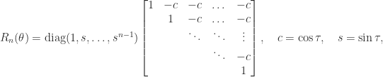
 , QR with column pivoting reorders
 ![A\Pi = [a_3,~a_4,~a_2,~a_1]](https://s0.wp.com/latex.php?latex=A%5CPi+%3D+%5Ba_3%2C%7Ea_4%2C%7Ea_2%2C%7Ea_1%5D&bg=ffffff&fg=222222&s=0&c=20201002) and yields
and yields  for
for  (say). In fact, this factorization provides a very good RRF, as in
  we have
  .
.  factorization
 ![\notag R = \begin{array}[b]{@{\mskip33mu}c@{\mskip-16mu}c@{\mskip-10mu}c@{}} \scriptstyle k & \scriptstyle n-k & \\ \multicolumn{2}{c}{ \left[\begin{array}{c@{~}c@{~}} R_{11}& R_{12} \\ 0 & R_{22} \\ \end{array}\right]} & \mskip-12mu\ \begin{array}{c} \scriptstyle k \\ \scriptstyle n-k \end{array} \end{array}. \qquad (6)](https://s0.wp.com/latex.php?latex=%5Cnotag++++R+%3D++++%5Cbegin%7Barray%7D%5Bb%5D%7B%40%7B%5Cmskip33mu%7Dc%40%7B%5Cmskip-16mu%7Dc%40%7B%5Cmskip-10mu%7Dc%40%7B%7D%7D++++%5Cscriptstyle+k+%26++++%5Cscriptstyle+n-k+%26++++%5C%5C++++%5Cmulticolumn%7B2%7D%7Bc%7D%7B++++++++%5Cleft%5B%5Cbegin%7Barray%7D%7Bc%40%7B%7E%7Dc%40%7B%7E%7D%7D++++++++++++++++++R_%7B11%7D%26+R_%7B12%7D+%5C%5C++++++++++++++++++++0+++%26+R_%7B22%7D+%5C%5C++++++++++++++%5Cend%7Barray%7D%5Cright%5D%7D++++%26+%5Cmskip-12mu%5C++++++++++%5Cbegin%7Barray%7D%7Bc%7D++++++++++++++%5Cscriptstyle+k+%5C%5C++++++++++++++%5Cscriptstyle+n-k++++++++++++++%5Cend%7Barray%7D++++%5Cend%7Barray%7D.+%5Cqquad+%286%29+&bg=ffffff&fg=222222&s=0&c=20201002)

 to zero gives a rank-
 . We would like to be able to detect this situation from
 and minimize
  .
.  the approximations in (9) can hold to within a factor
  .
.  and
and  , where
  .
.  , with
  and let
  be such that
  satisfies
  . Then if
 , which yields the result.
 ![\Pi = [\Pi_1~\pi]](https://s0.wp.com/latex.php?latex=%5CPi+%3D+%5B%5CPi_1%7E%5Cpi%5D&bg=ffffff&fg=222222&s=0&c=20201002) , where
, where  , and partition
 . Then
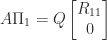
 . On the other hand, if
  is an SVD with
  ,
,  , and
, and ![V = [V_1~v]](https://s0.wp.com/latex.php?latex=V+%3D+%5BV_1%7Ev%5D&bg=ffffff&fg=222222&s=0&c=20201002) then
then 

 as
as 

 , as required.

 .
.  to the bottom of
  columns of the matrix of right singular vectors.
  , but it does not provide an efficient algorithm for computing one.
  flops.
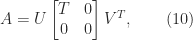
 is upper triangular and
  upper triangular or lower triangular a UTV decomposition and he defines a rank-revealing UTV decomposition of numerical rank

 and
and  are permutation matrices,
  and
and  are
are  lower and
  and
and  are
are  . Analogously to (7) and (8), we always have
  and
and  . With a suitable pivoting strategy we can hope that
  and
and  .
.  . This is analogue for LU factorization of Theorem 2.
 ![\notag \Pi_1 A \Pi_2 = LU = \begin{bmatrix} L_{11} & 0 \\ L_{12} & I_{m-k,n-k} \end{bmatrix} \begin{array}[b]{@{\mskip33mu}c@{\mskip-16mu}c@{\mskip-10mu}c@{}} \scriptstyle k & \scriptstyle n-k & \\ \multicolumn{2}{c}{ \left[\begin{array}{c@{~}c@{~}} U_{11}& U_{12} \\ 0 & U_{22} \\ \end{array}\right]} & \mskip-12mu\ \begin{array}{c} \scriptstyle k \\ \scriptstyle n-k \end{array} \end{array},](https://s0.wp.com/latex.php?latex=%5Cnotag+++++%5CPi_1+A+%5CPi_2+%3D+LU+%3D+++++%5Cbegin%7Bbmatrix%7D+++++L_%7B11%7D+%26++0++++%5C%5C+++++L_%7B12%7D+%26+I_%7Bm-k%2Cn-k%7D+++++%5Cend%7Bbmatrix%7D++++%5Cbegin%7Barray%7D%5Bb%5D%7B%40%7B%5Cmskip33mu%7Dc%40%7B%5Cmskip-16mu%7Dc%40%7B%5Cmskip-10mu%7Dc%40%7B%7D%7D++++%5Cscriptstyle+k+%26++++%5Cscriptstyle+n-k+%26++++%5C%5C++++%5Cmulticolumn%7B2%7D%7Bc%7D%7B++++++++%5Cleft%5B%5Cbegin%7Barray%7D%7Bc%40%7B%7E%7Dc%40%7B%7E%7D%7D++++++++++++++++++U_%7B11%7D%26+U_%7B12%7D+%5C%5C++++++++++++++++++++0+++%26+U_%7B22%7D+%5C%5C++++++++++++++%5Cend%7Barray%7D%5Cright%5D%7D++++%26+%5Cmskip-12mu%5C++++++++++%5Cbegin%7Barray%7D%7Bc%7D++++++++++++++%5Cscriptstyle+k+%5C%5C++++++++++++++%5Cscriptstyle+n-k++++++++++++++%5Cend%7Barray%7D++++%5Cend%7Barray%7D%2C+&bg=ffffff&fg=222222&s=0&c=20201002)

 .
. 
 ), the
  .. However, with complete pivoting we obtain
  and
and  .
.  math mode

 is a factorization
  , where
  and
and  are unitary and
  , with
  to specify the matrix to which the singular value belongs.
 or
or  , whose eigenvalues are the squares of the singular values of
 zero eigenvalues if
  .
. ,
,
 .
.

 (the equality case in the Cauchy–Schwarz inequality). For example, (2) is equivalent to
 ,
,
 and nonsingular
  and
and  ,
,
 .
.
 . The bounds (5) and (6) are intuitively reasonable, because unitary transformations preserve singular values and the bounds quantify in different ways how close
  , and
, and  . Then
 if
if  .
. is the leading principal submatrix of order
  ).
). and
and  , so that
  and
and
 , so
, so  and
and
 . However, when
  may be less than the smallest singular value of
 ![A = [A_{11}~A_{12}]](https://s0.wp.com/latex.php?latex=A+%3D+%5BA_%7B11%7D%7EA_%7B12%7D%5D&bg=ffffff&fg=222222&s=0&c=20201002) then
then  for all
  for which the left-hand side is defined.
 is pseudo-orthogonal if
 is a signature matrix. A matrix
  -orthogonal matrix, where
  then
then  is also pseudo-orthogonal. Furthermore,
 is orthogonal, this equation implies that
  and hence that
 and
and ![\Sigma = \left[\begin{smallmatrix}1 & 0 \\ 0 & -1 \end{smallmatrix}\right]](https://s0.wp.com/latex.php?latex=%5CSigma+%3D+%5Cleft%5B%5Cbegin%7Bsmallmatrix%7D1+%26+0+%5C%5C+0+%26+-1+%5Cend%7Bsmallmatrix%7D%5Cright%5D&bg=ffffff&fg=222222&s=0&c=20201002) ,
, 

 .
. is an eigenvalue of
  is also an eigenvalue and it has the same algebraic and geometric multiplicities as
 , which means that
  , and any such orthogonal matrix is pseudo-orthogonal.
 of a symmetric positive definite
  and want the Cholesky factorization of
  , which is assumed to be symmetric positive definite. A more general downdating problem is that we are given
![\notag A = \begin{array}[b]{cc} \left[\begin{array}{@{}c@{}} A_1\\ A_2 \end{array}\right] & \mskip-22mu\ \begin{array}{l} \scriptstyle p \\ \scriptstyle q \end{array} \end{array}, \quad p\ge n,](https://s0.wp.com/latex.php?latex=%5Cnotag+++A+%3D+%5Cbegin%7Barray%7D%5Bb%5D%7Bcc%7D++++++++%5Cleft%5B%5Cbegin%7Barray%7D%7B%40%7B%7Dc%40%7B%7D%7D++++++++++++++++++A_1%5C%5C++++++++++++++++++A_2++++++++++++++%5Cend%7Barray%7D%5Cright%5D++++++++%26+%5Cmskip-22mu%5C++++++++++%5Cbegin%7Barray%7D%7Bl%7D++++++++++++++%5Cscriptstyle+p+%5C%5C++++++++++++++%5Cscriptstyle+q++++++++++%5Cend%7Barray%7D++++%5Cend%7Barray%7D%2C++++%5Cquad+p%5Cge+n%2C+&bg=ffffff&fg=222222&s=0&c=20201002)
 and wish to obtain the Cholesky factor
  of
of  . Note that
  ). Assuming that
  , we would like to obtain
  . If we can find a pseudo-orthogonal matrix
 upper triangular, then
 hyperbolic rotation has the form (4), and an
  hyperbolic rotation embedded in it at the intersection of rows and columns
  , for some
  and
and  has the form
 ![QA = \left[\begin{smallmatrix} R \\ 0 \end{smallmatrix}\right]](https://s0.wp.com/latex.php?latex=QA+%3D+%5Cleft%5B%5Cbegin%7Bsmallmatrix%7D+R+%5C%5C+0+%5Cend%7Bsmallmatrix%7D%5Cright%5D&bg=ffffff&fg=222222&s=0&c=20201002) with
with  and
and  upper triangular. The factorization exists if
  is positive definite.
 are given, and
  . For
. For  or
or  we have the standard least squares (LS) problem and the quadratic form is definite, while for
  the problem is to minimize a genuinely indefinite quadratic form. This problem arises, for example, in the area of optimization known as
  smoothing.
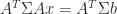 , and since the Hessian matrix of the quadratic objective function in (7) is
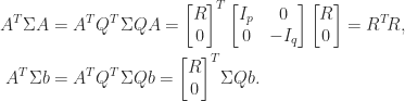
 , where
  comprises the first
  . The same equation can also be obtained without using the normal equations by substituting the hyperbolic QR factorization into (7).
 with
with  , partition
![\notag A = \mskip5mu \begin{array}[b]{@{\mskip-20mu}c@{\mskip0mu}c@{\mskip-1mu}c@{}} & \mskip10mu\scriptstyle p & \scriptstyle q \\ \mskip15mu \begin{array}{r} \scriptstyle p \\ \scriptstyle q \end{array}~ & \multicolumn{2}{c}{\mskip-15mu \left[\begin{array}{c@{~}c@{~}} A_{11} & A_{12}\\ A_{21} & A_{22} \end{array}\right] } \end{array}, \qquad (8)](https://s0.wp.com/latex.php?latex=%5Cnotag+++A++%3D+%5Cmskip5mu++++%5Cbegin%7Barray%7D%5Bb%5D%7B%40%7B%5Cmskip-20mu%7Dc%40%7B%5Cmskip0mu%7Dc%40%7B%5Cmskip-1mu%7Dc%40%7B%7D%7D++++%26+%5Cmskip10mu%5Cscriptstyle+p+%26+%5Cscriptstyle+q+%5C%5C+++++++%5Cmskip15mu++++++++++%5Cbegin%7Barray%7D%7Br%7D++++++++++++++%5Cscriptstyle+p+%5C%5C++++++++++++++%5Cscriptstyle+q++++++++++%5Cend%7Barray%7D%7E++++%26+++++++%5Cmulticolumn%7B2%7D%7Bc%7D%7B%5Cmskip-15mu++++++++++%5Cleft%5B%5Cbegin%7Barray%7D%7Bc%40%7B%7E%7Dc%40%7B%7E%7D%7D++++++++++++++++++A_%7B11%7D+%26+A_%7B12%7D%5C%5C++++++++++++++++++A_%7B21%7D+%26+A_%7B22%7D++++++++++++++++%5Cend%7Barray%7D%5Cright%5D+++++++%7D++++%5Cend%7Barray%7D%2C+%5Cqquad+%288%29+&bg=ffffff&fg=222222&s=0&c=20201002)
 is nonsingular. The exchange operator is defined by
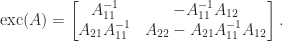


 .
. exists then
  .
.
 and then eliminating
 , we have
 there is a unique
  and
and  , which implies by (10) that
  , which implies that
  , it follows that
  also has a nonsingular
  block and so
  . But (9) shows that
  , and we conclude that
  exists and Lemma 1 shows that
  . Hence, using (9),
 be pseudo-orthogonal with respect to
 ![\notag Q = \begin{array}[b]{@{\mskip33mu}c@{\mskip-16mu}c@{\mskip-10mu}c@{}} \scriptstyle p & \scriptstyle n-p & \\ \multicolumn{2}{c}{ \left[\begin{array}{c@{~}c@{~}} Q_{11}& Q_{12} \\ Q_{21}& Q_{22} \\ \end{array}\right]} & \mskip-12mu\ \begin{array}{c} \scriptstyle p \\ \scriptstyle n-p \end{array} \end{array}, \quad p \le \displaystyle\frac{n}{2}.](https://s0.wp.com/latex.php?latex=%5Cnotag++++Q+%3D++++%5Cbegin%7Barray%7D%5Bb%5D%7B%40%7B%5Cmskip33mu%7Dc%40%7B%5Cmskip-16mu%7Dc%40%7B%5Cmskip-10mu%7Dc%40%7B%7D%7D++++%5Cscriptstyle+p+%26++++%5Cscriptstyle+n-p+%26++++%5C%5C++++%5Cmulticolumn%7B2%7D%7Bc%7D%7B++++++++%5Cleft%5B%5Cbegin%7Barray%7D%7Bc%40%7B%7E%7Dc%40%7B%7E%7D%7D++++++++++++++++++Q_%7B11%7D%26+Q_%7B12%7D+%5C%5C++++++++++++++++++Q_%7B21%7D%26+Q_%7B22%7D+%5C%5C++++++++++++++%5Cend%7Barray%7D%5Cright%5D%7D++++%26+%5Cmskip-12mu%5C++++++++++%5Cbegin%7Barray%7D%7Bc%7D++++++++++++++%5Cscriptstyle+p+%5C%5C++++++++++++++%5Cscriptstyle+n-p++++++++++++++%5Cend%7Barray%7D++++%5Cend%7Barray%7D%2C+%5Cquad+p+%5Cle+%5Cdisplaystyle%5Cfrac%7Bn%7D%7B2%7D.+&bg=ffffff&fg=222222&s=0&c=20201002)
 and
and  such that
![\notag \begin{bmatrix} U_1^T & 0\\ 0 & U_2^T \end{bmatrix} \begin{bmatrix} Q_{11} & Q_{12}\\ Q_{21} & Q_{22} \end{bmatrix} \begin{bmatrix} V_1 & 0\\ 0 & V_2 \end{bmatrix} = \begin{array}[b]{@{\mskip35mu}c@{\mskip30mu}c@{\mskip-10mu}c@{}c} \scriptstyle p & \scriptstyle p & \scriptstyle n-2p & \\ \multicolumn{3}{c}{ \left[\begin{array}{c@{~}|c@{~}c} C & -S & 0 \\ \hline -S & C & 0 \\ 0 & 0 & I_{n-2p} \end{array}\right]} & \mskip-12mu \begin{array}{c} \scriptstyle p \\ \scriptstyle p \\ \scriptstyle n-2p \end{array} \end{array}, \qquad (11)](https://s0.wp.com/latex.php?latex=%5Cnotag++++%5Cbegin%7Bbmatrix%7D++U_1%5ET+%26+0%5C%5C++++++++++++++++++++++++++0+++%26+U_2%5ET++++%5Cend%7Bbmatrix%7D++++%5Cbegin%7Bbmatrix%7D++Q_%7B11%7D+%26+Q_%7B12%7D%5C%5C++++++++++++++++++++++++++Q_%7B21%7D+%26+Q_%7B22%7D++++%5Cend%7Bbmatrix%7D++++%5Cbegin%7Bbmatrix%7D++V_1+%26+0%5C%5C++++++++++++++++++++++++++0+++%26+V_2++++%5Cend%7Bbmatrix%7D++++%3D++++%5Cbegin%7Barray%7D%5Bb%5D%7B%40%7B%5Cmskip35mu%7Dc%40%7B%5Cmskip30mu%7Dc%40%7B%5Cmskip-10mu%7Dc%40%7B%7Dc%7D++++%5Cscriptstyle+p+%26++++%5Cscriptstyle+p+%26++++%5Cscriptstyle+n-2p+%26++++%5C%5C++++%5Cmulticolumn%7B3%7D%7Bc%7D%7B++++%5Cleft%5B%5Cbegin%7Barray%7D%7Bc%40%7B%7E%7D%7Cc%40%7B%7E%7Dc%7D++++C+%26+++-S++++++%26+0+++%5C%5C++++%5Chline+++-S+%26++++C++++++%26+0+++%5C%5C++++0+%26++++0++++++%26+I_%7Bn-2p%7D++++%5Cend%7Barray%7D%5Cright%5D%7D++++%26+%5Cmskip-12mu++++%5Cbegin%7Barray%7D%7Bc%7D++++%5Cscriptstyle+p+%5C%5C++++%5Cscriptstyle+p+%5C%5C++++%5Cscriptstyle+n-2p++++%5Cend%7Barray%7D++++%5Cend%7Barray%7D%2C+%5Cqquad+%2811%29+&bg=ffffff&fg=222222&s=0&c=20201002)
 ,
,  , and
, and  , with
  for all
  .
.![\left[\begin{smallmatrix}C & -S \\ -S & C \end{smallmatrix}\right]](https://s0.wp.com/latex.php?latex=%5Cleft%5B%5Cbegin%7Bsmallmatrix%7DC+%26+-S+%5C%5C+-S+%26+C+%5Cend%7Bsmallmatrix%7D%5Cright%5D&bg=ffffff&fg=222222&s=0&c=20201002) in (11) generalizes the
in (11) generalizes the 
 for all
  singular values occur in reciprocal pairs, hence the largest and smallest singular values satisfy
  (with strict inequality unless
  ). This gives another proof of (3).
 for
for  . More results for pseudo-orthogonal matrices can be obtained as special cases of results for automorphism groups of general scalar products. See, for example, Mackey, Mackey, and Tisseur (2006).
 the set of pseudo-orthogonal matrices is known to have four connected components, a topological property that can be proved using the hyperbolic CS decomposition (Motlaghian, Armandnejad, and Hall, 2018).
 such that
  . These correspond to the automorphism group of the scalar product
  for
for  . The results we have discussed generalize in a straightforward way to pseudo-unitary matrices.
 , where
 ![\notag \left[\begin{array}{rrrr} 3 & -1 & 1 & 1\\ -1 & 3 & 1 & -1\\ -1 & -1 & 3 & 1\\ 1 & 1 & 1 & 3 \end{array}\right] = \left[\begin{array}{rrrr} 1 & 0 & 0 & 0\\ -\frac{1}{3} & 1 & 0 & 0\\ -\frac{1}{3} & -\frac{1}{2} & 1 & 0\\ \frac{1}{3} & \frac{1}{2} & 0 & 1 \end{array}\right] \left[\begin{array}{rrrr} 3 & -1 & 1 & 1\\ 0 & \frac{8}{3} & \frac{4}{3} & -\frac{2}{3}\\ 0 & 0 & 4 & 1\\ 0 & 0 & 0 & 3 \end{array}\right]. \qquad (1)](https://s0.wp.com/latex.php?latex=%5Cnotag++++%5Cleft%5B%5Cbegin%7Barray%7D%7Brrrr%7D++++++3+%26+-1+%26+1+%26+1%5C%5C+++++-1+%26+3+%26+1+%26+-1%5C%5C+++++-1+%26+-1+%26+3+%26+1%5C%5C++++++1+%26+1+%26+1+%26+3++++%5Cend%7Barray%7D%5Cright%5D+++%3D++++%5Cleft%5B%5Cbegin%7Barray%7D%7Brrrr%7D+++++1+%26+0+%26+0+%26+0%5C%5C++++-%5Cfrac%7B1%7D%7B3%7D+%26+1+%26+0+%26+0%5C%5C++++-%5Cfrac%7B1%7D%7B3%7D+%26+-%5Cfrac%7B1%7D%7B2%7D+%26+1+%26+0%5C%5C+++++%5Cfrac%7B1%7D%7B3%7D+%26+%5Cfrac%7B1%7D%7B2%7D+%26+0+%26+1++++%5Cend%7Barray%7D%5Cright%5D++++%5Cleft%5B%5Cbegin%7Barray%7D%7Brrrr%7D++++3+%26+-1+%26+1+%26+1%5C%5C++++0+%26+%5Cfrac%7B8%7D%7B3%7D+%26+%5Cfrac%7B4%7D%7B3%7D+%26+-%5Cfrac%7B2%7D%7B3%7D%5C%5C++++0+%26+0+%26+4+%26+1%5C%5C++++0+%26+0+%26+0+%26+3++++%5Cend%7Barray%7D%5Cright%5D.+%5Cqquad+%281%29+&bg=ffffff&fg=222222&s=0&c=20201002)
 reduces to solving the triangular systems
  and
and  , since then
  .
. the leading principal submatrix of
  . If
. If  then the factorization may exist, but if so it is not unique.
 then the
  are necessarily nonsingular and so
  . The left side of this equation is unit lower triangular and the right side is upper triangular; therefore both sides must equal the identity matrix, which means that
  and
and  , as required.
 , which implies that
  . Hence
  . In fact, such determinantal formulas hold for all the elements of
 ![\notag \begin{aligned} \ell_{ij} &= \frac{ \det\bigl( A( [1:j-1, \, i], 1:j ) \bigr) }{ \det( A_j ) }, \quad i > j, \\ u_{ij} &= \frac{ \det\bigl( A( 1:i, [1:i-1, \, j] ) \bigr) } { \det( A_{i-1} ) }, \quad i \le j. \end{aligned}](https://s0.wp.com/latex.php?latex=%5Cnotag++++%5Cbegin%7Baligned%7D++++%5Cell_%7Bij%7D+%26%3D+%5Cfrac%7B+%5Cdet%5Cbigl%28+A%28+%5B1%3Aj-1%2C+%5C%2C+i%5D%2C+1%3Aj+%29+%5Cbigr%29+%7D%7B+%5Cdet%28+A_j+%29+%7D%2C+++++++++++++%5Cquad+i+%3E+j%2C+%5C%5C++++u_%7Bij%7D+%26%3D+%5Cfrac%7B+%5Cdet%5Cbigl%28+A%28+1%3Ai%2C+%5B1%3Ai-1%2C+%5C%2C+j%5D+%29+%5Cbigr%29+%7D+++++++++++++++++++%7B+%5Cdet%28+A_%7Bi-1%7D+%29+%7D%2C+++++++++++++%5Cquad+i+%5Cle+j.++++%5Cend%7Baligned%7D+&bg=ffffff&fg=222222&s=0&c=20201002)
 , where
  and
and  are vectors of subscripts, denotes the submatrix formed from the intersection of the rows indexed by
  to upper triangular form
  in
in  stages. At the
 are the multipliers. Of course each
  must be nonzero for these formulas to be defined, and this is connected with the conditions of Theorem 1, since
  . The final
  for
for  , and
, and  for
for  , that is, the multipliers make up the
  we can just solve
  and
and  , re-using the LU factorization. Similarly, solving
  reduces to solving the triangular systems
  and
and  .
. then determines the first column of
  . This leads to the Doolittle method, which involves inner products of partial rows of
 ordering of the loops in the factorization is the basis of early Fortran implementations of LU factorization, such as that in LINPACK. The inner loop travels down the columns of
  ordering, which updates the matrix a row at a time, and is appropriate for a language such as C that stores arrays by row.
 and
and  orderings correspond to the Doolittle method. The last two of the
  orderings are the
  and
and  orderings, to which we will return later.
 we can write
 matrix
  is called the Schur complement of
  in
in  and
and  have the correct forms for a unit lower triangular matrix and an upper triangular matrix, respectively. If we can find an LU factorization
  then
then
 . If we can show that the Schur complement inherits the same structure then it follows by induction that we can compute the factorization for
  and
and  -matrices,
 if
if  for
for  and lower bandwidth
  if
if  . Another use of (2) is to show that
  and
and  have only
  :
:
 . This leads to the following algorithm:
 .
. for
for  .
. for
for  .
. .
. .
. partitioning, in which we assume we have already computed the first block column of
 .
. for
for  .
. —
— .
. lower triangular and
  , where
![\notag A = \left[ \begin{array}{rr|rr} 0 & 1 & 1 & 1 \\ -1 & 1 & 1 & 1 \\\hline -2 & 3 & 4 & 2 \\ -1 & 2 & 1 & 3 \\ \end{array} \right] = \left[ \begin{array}{cc|cc} 1 & 0 & 0 & 0 \\ 0 & 1 & 0 & 0 \\\hline 1 & 2 & 1 & 0 \\ 1 & 1 & 0 & 1 \\ \end{array} \right] \left[ \begin{array}{rr|rr} 0 & 1 & 1 & 1 \\ -1 & 1 & 1 & 1 \\\hline 0 & 0 & 1 & -1 \\ 0 & 0 & -1 & 1 \\ \end{array} \right].](https://s0.wp.com/latex.php?latex=%5Cnotag+++++A+%3D++++++%5Cleft%5B+%5Cbegin%7Barray%7D%7Brr%7Crr%7D++++++0++%26++1++%26++1++%26++1++%5C%5C+++++-1++%26++1++%26++1++%26++1++%5C%5C%5Chline+++++-2++%26++3++%26++4++%26++2++%5C%5C+++++-1++%26++2++%26++1++%26++3++%5C%5C+++++++++++++%5Cend%7Barray%7D++++++%5Cright%5D++++++%3D++++++%5Cleft%5B+%5Cbegin%7Barray%7D%7Bcc%7Ccc%7D++++++1++%26++0++%26++0++%26++0++%5C%5C++++++0++%26++1++%26++0++%26++0++%5C%5C%5Chline++++++1++%26++2++%26++1++%26++0++%5C%5C++++++1++%26++1++%26++0++%26++1++%5C%5C+++++++++++++%5Cend%7Barray%7D++++++%5Cright%5D++++++%5Cleft%5B+%5Cbegin%7Barray%7D%7Brr%7Crr%7D++++++0++%26++1++%26++1++%26++1++%5C%5C+++++-1++%26++1++%26++1++%26++1++%5C%5C%5Chline++++++0++%26++0++%26++1++%26+-1++%5C%5C++++++0++%26++0++%26+-1++%26++1++%5C%5C+++++++++++++%5Cend%7Barray%7D++++++%5Cright%5D.+&bg=ffffff&fg=222222&s=0&c=20201002)
 submatrix. In the context of a linear system
  , we have effectively solved for the variables
  and
and  and then substituted for
  leading principal block submatrices of
  involving the diagonal blocks of
  an LU factorization
  exists. To first order, this equation is
  , which gives
 is strictly lower triangular and
  is upper triangular, we have, to first order,
 denotes the strictly lower triangular part and
  the strictly upper triangular part. Clearly, the sensitivity of the LU factors depends on the inverses of
  and
and  are numerically stable in the sense that
  with
with  , where
  is a constant and
![\notag \left[\begin{array}{rrr} 3 & -1 & -2\\ -2 & 3 & -1\\ -2 & -1 & 3 \end{array}\right] \qquad (1)](https://s0.wp.com/latex.php?latex=%5Cnotag++%5Cleft%5B%5Cbegin%7Barray%7D%7Brrr%7D+++++3+%26+-1+%26+-2%5C%5C++++-2+%26++3+%26+-1%5C%5C++++-2+%26+-1+%26++3+++%5Cend%7Barray%7D%5Cright%5D+%5Cqquad+%281%29+&bg=ffffff&fg=222222&s=0&c=20201002)
![[1~1~1]^T](https://s0.wp.com/latex.php?latex=%5B1%7E1%7E1%5D%5ET&bg=ffffff&fg=222222&s=0&c=20201002) is a null vector. A useful definition of a matrix with large diagonal requires a stronger property.
is a null vector. A useful definition of a matrix with large diagonal requires a stronger property.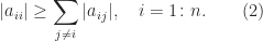
 is (strictly) diagonally dominant by rows.
 let
let  and choose
  . Then the

 and so
 square matrices. Irreducibility is equivalent to the directed graph of
  for some
  such that
  . Define

 ,
,
 is nonempty, because if it were empty then we would have
  for all
  , then putting
  , which is a contradiction. Hence as long as
  for some
  , we obtain
  , which contradicts the diagonal dominance. Therefore we must have
  for all
  . This means that all the rows indexed by
  have zeros in the columns indexed by
 ![\notag T_n = \left[\begin{array}{@{\mskip 5mu}c*{4}{@{\mskip 15mu} r}@{\mskip 5mu}} 2 & -1 & & & \\ -1 & 2 & -1 & & \\ & -1 & 2 & \ddots & \\ & & \ddots & \ddots & -1\\ & & & -1 & 2 \end{array}\right], \qquad (5)](https://s0.wp.com/latex.php?latex=%5Cnotag++T_n+%3D+%5Cleft%5B%5Cbegin%7Barray%7D%7B%40%7B%5Cmskip+5mu%7Dc%2A%7B4%7D%7B%40%7B%5Cmskip+15mu%7D+r%7D%40%7B%5Cmskip+5mu%7D%7D++++++2+%26+++-1++%26++++++++++%26+++++++++%26+%5C%5C+++++-1+%26++++2++%26++-1++++++%26+++++++++%26+%5C%5C++++++++%26++++-1+%26+++2++++++%26++%5Cddots+%26+%5C%5C++++++++%26+++++++%26++%5Cddots++%26++%5Cddots+%26+-1%5C%5C++++++++%26+++++++%26++++++++++%26++-1+++++%26+2++++++++++++%5Cend%7Barray%7D%5Cright%5D%2C+%5Cqquad+%285%29+&bg=ffffff&fg=222222&s=0&c=20201002)
 or
or  by
by 
 and
and
 and
and  have the same nonzero eigenvalues, we conclude that
  , where
  denotes the spectrum. Hence
  is symmetric positive definite and
  is singular and symmetric positive semidefinite.
 is singular and hence cannot be strictly diagonally dominant, by Theorem 1. So
 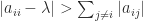 cannot be true for all
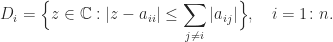
 , so
, so  , so the eigenvalues are nonnegative, and hence positive since nonzero. This provides another proof that the matrix

 is diagonally dominant by rows for some diagonal matrix
  with
with  for all
 , defined by
 partitioning
  , the diagonal blocks
  are all nonsingular and
 then block diagonal dominance reduces to the usual notion of diagonal dominance. Block diagonal dominance holds for certain block tridiagonal matrices arising in the discretization of PDEs.
 .
. . Let
. Let  satisfy
  and let
  . The result is obtained on applying this bound to
  .
.  , where
  ,
,  , and
, and  for
for  . It is easy to see that
  , which gives another proof that
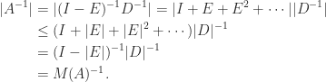
 , so in view of its sign pattern
  .
.
 .
. satisfies
  for all
  . Let
. Let  . Taking absolute values in
  gives
gives
 , since
  . This inequality holds for all
  , which gives the result.