The Sylvester equation is the linear matrix equation

where 


In the case where 

so a solution can exist only when 
To determine when the Sylvester equation has a solution we will transform it into a simpler form. Let 


which is a Sylvester equation with upper triangular coefficient matrices. Equating the 

As long as the triangular matrices 


Since the Sylvester is a linear equation it must be possible to express it in the standard form “

where 

so the coefficient matrix is nonsingular when 
By considering the derivative of 


is the unique solution of 
Applications
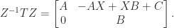
An important application of the Sylvester equation is in block diagonalization. Consider the block upper triangular matrix

If we can find a nonsingular matrix 


so computing 


and noting that 
Hence 

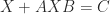
For another way in which Sylvester equations arises consider the expansion 


Sylvester equations also arise in the Schur–Parlett algorithm for computing matrix functions, which reduces a matrix to triangular Schur form 

Solution Methods
How can we solve the Sylvester equation? One possibility is to solve 


sylvester.
In recent years research has focused particularly on solving Sylvester equations in which
Sensitivity and the Separation
Define the separation of

The separation is positive if

so

It is not hard to show that 


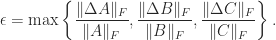
The separation features in a perturbation bound for the Sylvester equation. If

then
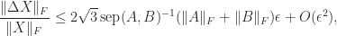
where
While we have the upper bound 


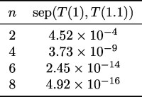
Even though the eigenvalues of 

The sep function was originally introduced by Stewart in the 1970s as a tool for studying the sensitivity of invariant subspaces.
Variations and Generalizations
The Sylvester equation has many variations and special cases, including the Lyapunov equation 

For 


References
This is a minimal set of references, which contain further useful references within.
- Peter Lancaster, Explicit Solutions of Linear Matrix Equations, SIAM Review, 12(4), 544–566, 1970.
- Nicholas J. Higham, Accuracy and Stability of Numerical Algorithms, second edition, Society for Industrial and Applied Mathematics, Philadelphia, PA, USA, 2002. Chapter 16.
- Nicholas J. Higham, Functions of Matrices: Theory and Computation, Society for Industrial and Applied Mathematics, Philadelphia, PA, USA, 2008.
- J. M. Varah, On the Separation of Two Matrices, SIAM J. Numer. Anal. 16 (2), 216–222, 1979.
Related Blog Posts
This article is part of the “What Is” series, available from https://nhigham.com/category/what-is and in PDF form from the GitHub repository https://github.com/higham/what-is.

Thank you for this post, I bumped into Sylvester equation while modelling biological oscillators as linear time invariant systems. If you have a set of aligned time series for different entities, each one periodical, you can transform in frequency domain and convert the ODE system into a matrix equation, which was the Sylvester equation. After finding this I could find solutions and characterise the entities of the equation. I am sure the latter is trivial for people doing control, for me it was the key to get my method to work.