Care is needed when dealing with multivalued functions because identities that hold for positive scalars can fail in the complex plane. For example, it is not always true that 


![(-\pi,\pi]](https://s0.wp.com/latex.php?latex=%28-%5Cpi%2C%5Cpi%5D&bg=ffffff&fg=222222&s=0&c=20201002)
A powerful tool for dealing with multivalued complex functions is the unwinding number, defined for 
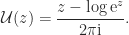
The unwinding number provides a correction term for the putative identity 

for all 
A useful formula for the unwinding number is
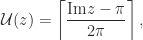
where 

![\mathrm{Im} z \in (-\pi, \pi]](https://s0.wp.com/latex.php?latex=%5Cmathrm%7BIm%7D+z+%5Cin+%28-%5Cpi%2C+%5Cpi%5D&bg=ffffff&fg=222222&s=0&c=20201002)
The unwinding number provides correction terms for various identities. For example, for 


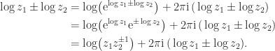
This gives the identities

Note that in textbooks one can find identities such as 

An application of the unwinding number to matrix functions is in computing the logarithm of a 

![\notag f\left( \begin{bmatrix} \lambda_1 & t_{12} \\ 0 & \lambda_2 \end{bmatrix} \right) = \begin{bmatrix} f(\lambda_1) & t_{12} f[\lambda_1,\lambda_2] \\ 0 & f(\lambda_2) \end{bmatrix},](https://s0.wp.com/latex.php?latex=%5Cnotag+++++f%5Cleft%28+%5Cbegin%7Bbmatrix%7D++++++++++++++++++++++%5Clambda_1+%26+t_%7B12%7D++%5C%5C++++++++++++++++++++++++++++0+++%26+%5Clambda_2+++++++++++++%5Cend%7Bbmatrix%7D+%5Cright%29++++++++++%3D+%5Cbegin%7Bbmatrix%7D+++++++++++++++f%28%5Clambda_1%29+%26+t_%7B12%7D+f%5B%5Clambda_1%2C%5Clambda_2%5D+%5C%5C+++++++++++++++++0++++++++++%26+f%28%5Clambda_2%29+++++++++++++%5Cend%7Bbmatrix%7D%2C+&bg=ffffff&fg=222222&s=0&c=20201002)
where the divided difference
![\notag f[\lambda_1,\lambda_2] = \begin{cases} \displaystyle\frac{f(\lambda_2)-f(\lambda_1)}{\lambda_2-\lambda_1}, & \lambda_1 \ne \lambda_2, \\ f'(\lambda_1), & \lambda_1 = \lambda_2. \end{cases}](https://s0.wp.com/latex.php?latex=%5Cnotag+++f%5B%5Clambda_1%2C%5Clambda_2%5D++++%3D+%5Cbegin%7Bcases%7D++++++%5Cdisplaystyle%5Cfrac%7Bf%28%5Clambda_2%29-f%28%5Clambda_1%29%7D%7B%5Clambda_2-%5Clambda_1%7D%2C++++++%26+%5Clambda_1+%5Cne+%5Clambda_2%2C+%5C%5C++++++f%27%28%5Clambda_1%29%2C+%26+%5Clambda_1+%3D+%5Clambda_2.+++++%5Cend%7Bcases%7D+&bg=ffffff&fg=222222&s=0&c=20201002)
When 

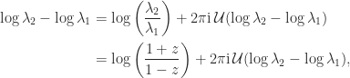
where 

we obtain
![\notag f[\lambda_1,\lambda_2] = \displaystyle\frac{2\mathrm{atanh}(z) + 2\pi \mathrm{i}\, \mathcal{U}(\log \lambda_2 - \log \lambda_1)}{\lambda_2-\lambda_1}, \quad \lambda_1 \ne \lambda_2.](https://s0.wp.com/latex.php?latex=%5Cnotag+++f%5B%5Clambda_1%2C%5Clambda_2%5D++++%3D+%5Cdisplaystyle%5Cfrac%7B2%5Cmathrm%7Batanh%7D%28z%29+%2B+2%5Cpi+%5Cmathrm%7Bi%7D%5C%2C++++++%5Cmathcal%7BU%7D%28%5Clog+%5Clambda_2+-+%5Clog+%5Clambda_1%29%7D%7B%5Clambda_2-%5Clambda_1%7D%2C++++%5Cquad+%5Clambda_1+%5Cne+%5Clambda_2.+&bg=ffffff&fg=222222&s=0&c=20201002)
Assuming that we have an accurate 
![f[\lambda_1,\lambda_2]](https://s0.wp.com/latex.php?latex=f%5B%5Clambda_1%2C%5Clambda_2%5D&bg=ffffff&fg=222222&s=0&c=20201002)

logm.
Matrix Unwinding Function
The unwinding number leads to the matrix unwinding function, defined for 

Here, 

![(-\pi, \pi]](https://s0.wp.com/latex.php?latex=%28-%5Cpi%2C+%5Cpi%5D&bg=ffffff&fg=222222&s=0&c=20201002)

As an example, the matrix
![\notag A = \left[\begin{array}{rrrr} 3 & 1 & -1 & -9\\ -1 & 3 & 9 & -1\\ -1 & -9 & 3 & 1\\ 9 & -1 & -1 & 3 \end{array}\right], \quad \Lambda(A) = \{ 2\pm 8\mathrm{i}, 4 \pm 10\mathrm{i} \}](https://s0.wp.com/latex.php?latex=%5Cnotag+++A+%3D+%5Cleft%5B%5Cbegin%7Barray%7D%7Brrrr%7D++++3+%26+1+%26+-1+%26+-9%5C%5C++++-1+%26+3+%26+9+%26+-1%5C%5C++++-1+%26+-9+%26+3+%26+1%5C%5C++++9+%26+-1+%26+-1+%26+3+%5Cend%7Barray%7D%5Cright%5D%2C++++%5Cquad+%5CLambda%28A%29+%3D+%5C%7B+2%5Cpm+8%5Cmathrm%7Bi%7D%2C+4+%5Cpm+10%5Cmathrm%7Bi%7D+%5C%7D+&bg=ffffff&fg=222222&s=0&c=20201002)
has unwinding matrix function
![\notag X = \mathcal{U}(A) = \mathrm{i} \left[\begin{array}{rrrr} 0 & -\frac{1}{2} & 0 & \frac{3}{2}\\ \frac{1}{2} & 0 & -\frac{3}{2} & 0\\ 0 & \frac{3}{2} & 0 & -\frac{1}{2}\\ -\frac{3}{2} & 0 & \frac{1}{2} & 0 \end{array}\right], \quad \Lambda(X) = \{ \pm 1, \pm 2 \}.](https://s0.wp.com/latex.php?latex=%5Cnotag+++X+%3D+%5Cmathcal%7BU%7D%28A%29+%3D+%5Cmathrm%7Bi%7D+%5Cleft%5B%5Cbegin%7Barray%7D%7Brrrr%7D++++0+%26+-%5Cfrac%7B1%7D%7B2%7D+%26+0+%26+%5Cfrac%7B3%7D%7B2%7D%5C%5C++++%5Cfrac%7B1%7D%7B2%7D+%26+0+%26+-%5Cfrac%7B3%7D%7B2%7D+%26+0%5C%5C++++0+%26+%5Cfrac%7B3%7D%7B2%7D+%26+0+%26+-%5Cfrac%7B1%7D%7B2%7D%5C%5C++++-%5Cfrac%7B3%7D%7B2%7D+%26+0+%26+%5Cfrac%7B1%7D%7B2%7D+%26+0+%5Cend%7Barray%7D%5Cright%5D%2C++++%5Cquad+%5CLambda%28X%29+%3D+%5C%7B+%5Cpm+1%2C+%5Cpm+2+%5C%7D.+&bg=ffffff&fg=222222&s=0&c=20201002)
In general, if 
The matrix unwinding function is useful for providing correction terms for matrix identities involving multivalued functions. Here are four useful matrix identities, along with cases in which the correction term vanishes. See Aprahamian and Higham (2014) for proofs.
- For nonsingular
,
If
is an integer then the correction term is
. If
and
then
and so
and this equation is obviously true for
, too.
- If
are nonsingular and
then
If
for every eigenvalue
of
of
.
- If
,
If
is an integer or the eigenvalues of
then
.
- For nonsingular
If
, and this equation also holds for

![\notag (A^\alpha)^{1/\alpha} = A, \quad \alpha \in [-1,1],](https://s0.wp.com/latex.php?latex=%5Cnotag++++++%28A%5E%5Calpha%29%5E%7B1%2F%5Calpha%7D+%3D+A%2C+%5Cquad+%5Calpha+%5Cin+%5B-1%2C1%5D%2C++++&bg=ffffff&fg=222222&s=0&c=20201002)


The matrix unwinding function can be computed by an adaptation of the Schur–Parlett algorithm. The algorithm computes a Schur decomposition and re-orders it into a block form with eigenvalues having the same unwinding number in the same diagonal block. The unwinding function of each diagonal block is then a multiple of the identity and the off-diagonal blocks are obtained by the block Parlett recurrence. This approach gives more accurate results than directly evaluating unwindm is available at https://github.com/higham/unwinding
Matrix Argument Reduction
The matrix unwinding function can be of use computationally for reducing the size of the imaginary parts of the eigenvalues of a matrix. The function

has eigenvalues 
![\mathrm{Im} \lambda \in(-\pi,\pi]](https://s0.wp.com/latex.php?latex=%5Cmathrm%7BIm%7D+%5Clambda+%5Cin%28-%5Cpi%2C%5Cpi%5D&bg=ffffff&fg=222222&s=0&c=20201002)


Round Trip Relations
If you apply a matrix function and then its inverse do you get back to where you started, that is, is 


Here, 

History
The unwinding number was introduced by Corless, Hare and Jeffrey in 1996, to help implement computer algebra over the complex numbers. It was generalized to the matrix case by Aprahamian and Higham (2014).
References
This is a minimal set of references, which contain further useful references within.
- Mary Aprahamian and Nicholas J. Higham, The Matrix Unwinding Function, with an Application to Computing the Matrix Exponential, SIAM J. Matrix Anal. Appl. 35(1), 88–109, 2014.
- Mary Aprahamian and Nicholas J. Higham, Matrix Inverse Trigonometric and Inverse Hyperbolic Functions: Theory and Algorithms, SIAM J. Matrix Anal. Appl. 37(4), 1453–1477, 2016.
- Robert Corless and David Jeffrey, The Unwinding Number, SIGSAM Bull 30(2), 28–35, 1996.
- David Jeffrey, D. E. G. Hare and Robert Corless, Unwinding the Branches of the Lambert W Function, Math. Scientist 21, 1–7, 1996.
- Nicholas J. Higham, Functions of Matrices: Theory and Computation, Society for Industrial and Applied Mathematics, Philadelphia, PA, USA, 2008.
Related Blog Posts
- What Is a Matrix Function? (2020)
- What Is a Matrix Square Root? (2020)
- What Is the Matrix Logarithm? (2020)
- What Is the Matrix Exponential? (2020)
This article is part of the “What Is” series, available from https://nhigham.com/category/what-is and in PDF form from the GitHub repository https://github.com/higham/what-is.
