A symmetric indefinite matrix  is a symmetric matrix for which the quadratic form
  takes both positive and negative values. By contrast, for a positive definite matrix
  for all nonzero
  and for a negative definite matrix
  for all nonzero .
A neat way to express the indefinitess is that there exist vectors and  for which
 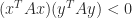 .
.
A symmetric indefinite matrix has both positive and negative eigenvalues and in some sense is a typical symmetric matrix. For example, a random symmetric matrix is usually indefinite:
>> rng(3); B = rand(4); A = B + B'; eig(A)'
ans =
  -8.9486e-01  -6.8664e-02   1.1795e+00   3.9197e+00
In general it is difficult to tell if a symmetric matrix is indefinite or definite, but there is one easy-to-spot sufficient condition for indefinitess: if the matrix has a zero diagonal element that has a nonzero element in its row then it is indefinite. Indeed if  then
then  , where
  is the
  th unit vector, so cannot be positive definite or negative definite. The existence of a nonzero element in the row of the zero rules out the matrix being positive semidefinite (
 for all ) or negative semidefinite (
 for all ).
An example of a symmetric indefinite matrix is a saddle point matrix, which has the block  form
form

where is symmetric positive definite and  . When is the identity matrix,
  is the augmented system matrix associated with a least squares problem
  . Another example is the
  reverse identity matrix
  , illustrated by
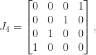
which has eigenvalues  (exercise: how many
  s and how many
  s?). A third example is a Toeplitz tridiagonal matrix with zero diagonal:
>> A = full(gallery('tridiag',5,1,0,1)), eig(sym(A))'
A =
     0     1     0     0     0
     1     0     1     0     0
     0     1     0     1     0
     0     0     1     0     1
     0     0     0     1     0
ans =
[-1, 0, 1, 3^(1/2), -3^(1/2)]
How can we exploit symmetry in solving a linear system  with a symmetric indefinite matrix ? A Cholesky factorization does not exist, but we could try to compute a factorization
  , where
  is unit lower triangular and
  is diagonal with both positive and negative diagonal entries. However, this factorization does not always exist and if it does, its computation in floating-point arithmetic can be numerically unstable. The simplest example of nonexistence is the matrix

The way round this is to allow to have  blocks. We can compute a block
  factorization
  , were
  is a permutation matrix, is unit lower triangular, and is block diagonal with diagonal blocks of size or
  . Various pivoting strategies, which determine , are possible, but the recommend one is the symmetric rook pivoting strategy of Ashcraft, Grimes, and Lewis (1998), which has the key property of producing a bounded factor. Solving now reduces to substitutions with and a solve with , which involves solving linear systems for the blocks and doing divisions for the
  blocks (scalars).
MATLAB implements factorization in its ldl function. Here is an example using Anymatrix:
>> A = anymatrix('core/blockhouse',4), [L,D,P] = ldl(A), eigA = eig(A)'
A =
  -4.0000e-01  -8.0000e-01  -2.0000e-01   4.0000e-01
  -8.0000e-01   4.0000e-01  -4.0000e-01  -2.0000e-01
  -2.0000e-01  -4.0000e-01   4.0000e-01  -8.0000e-01
   4.0000e-01  -2.0000e-01  -8.0000e-01  -4.0000e-01
L =
   1.0000e+00            0            0            0
            0   1.0000e+00            0            0
   5.0000e-01  -8.3267e-17   1.0000e+00            0
  -2.2204e-16  -5.0000e-01            0   1.0000e+00
D =
  -4.0000e-01  -8.0000e-01            0            0
  -8.0000e-01   4.0000e-01            0            0
            0            0   5.0000e-01  -1.0000e+00
            0            0  -1.0000e+00  -5.0000e-01
P =
     1     0     0     0
     0     1     0     0
     0     0     1     0
     0     0     0     1
eigA =
  -1.0000e+00  -1.0000e+00   1.0000e+00   1.0000e+00
Notice the blocks on the diagonal of , each of which contains one negative eigenvalue and one positive eigenvalue. The eigenvalues of are not the same as those of , but since and are congruent they have the same number of positive, zero, and negative eigenvalues.
References
- Cleve Ashcraft, Roger Grimes, and John Lewis, Accurate Symmetric Indefinite Linear Equation Solvers, SIAM J. Matrix Anal. Appl. 20, 513–561, 1998.
- Nicholas J. Higham and Mantas Mikaitis, Anymatrix: An Extendable MATLAB Matrix Collection, Numer. Algorithms, 90:3, 1175–1196, 2021.


 is diagonalizable if there exists a nonsingular matrix
  such that
  is diagonal. In other words, a diagonalizable matrix is one that is similar to a diagonal matrix.
 is equivalent to
  with
with  ,
,  , where
 ![X = [x_1,x_2,\dots, x_n]](https://s0.wp.com/latex.php?latex=X+%3D+%5Bx_1%2Cx_2%2C%5Cdots%2C+x_n%5D&bg=ffffff&fg=222222&s=0&c=20201002) . Hence
. Hence  ). A matrix with distinct eigenvalues is also diagonalizable.
 has distinct eigenvalues then it is diagonalizable.
 with corresponding eigenvectors
  . Suppose that
  for some
  . Then
 since
since  for
for  and
and  . Premultiplying
  by
by 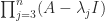 shows, in the same way, that
  . Continuing in this way we find that
  . Therefore the
  are linearly independent and hence
 ![\bigl[\begin{smallmatrix} 0 & 1 \\ 0 & 0 \end{smallmatrix}\bigr]](https://s0.wp.com/latex.php?latex=%5Cbigl%5B%5Cbegin%7Bsmallmatrix%7D+0+%26+1+%5C%5C+0+%26+0+%5Cend%7Bsmallmatrix%7D%5Cbigr%5D&bg=ffffff&fg=222222&s=0&c=20201002) . This matrix is a
. This matrix is a  , that is, any matrix in
  diagonalizable, where
  are nonzero? There are
  zero eigenvalues with eigenvectors any set of linearly independent vectors orthogonal to
  then
then  is the remaining eigenvalue, with eigenvector
  then all the eigenvalues of
 ![x = \bigl[{1 \atop 0} \bigr]](https://s0.wp.com/latex.php?latex=x+%3D+%5Cbigl%5B%7B1+%5Catop+0%7D+%5Cbigr%5D&bg=ffffff&fg=222222&s=0&c=20201002) and
and ![y = \bigl[{0 \atop 1} \bigr]](https://s0.wp.com/latex.php?latex=y+%3D+%5Cbigl%5B%7B0+%5Catop+1%7D+%5Cbigr%5D&bg=ffffff&fg=222222&s=0&c=20201002) , so
, so  is stochastic then
  , where
 ![e = [1,1,\dots,1]^T](https://s0.wp.com/latex.php?latex=e+%3D+%5B1%2C1%2C%5Cdots%2C1%5D%5ET&bg=ffffff&fg=222222&s=0&c=20201002) is the vector of ones. This means that
is the vector of ones. This means that  is an eigenvector of
 ![\notag \begin{aligned} A_n &= n^{-1}ee^T, \quad \textrm{in particular}~~ A_3 = \begin{bmatrix} \frac{1}{3} & \frac{1}{3} & \frac{1}{3}\\[3pt] \frac{1}{3} & \frac{1}{3} & \frac{1}{3}\\[3pt] \frac{1}{3} & \frac{1}{3} & \frac{1}{3} \end{bmatrix}, \qquad (1)\\ B_n &= \frac{1}{n-1}(ee^T -I), \quad \textrm{in particular}~~ B_3 = \begin{bmatrix} 0 & \frac{1}{2} & \frac{1}{2}\\[2pt] \frac{1}{2} & 0 & \frac{1}{2}\\[2pt] \frac{1}{2} & \frac{1}{2} & 0 \end{bmatrix}, \qquad (2)\\ C_n &= \begin{bmatrix} 1 & & & \\ \frac{1}{2} & \frac{1}{2} & & \\ \vdots & \vdots &\ddots & \\ \frac{1}{n} & \frac{1}{n} &\cdots & \frac{1}{n} \end{bmatrix}. \qquad (3)\\ \end{aligned}](https://s0.wp.com/latex.php?latex=%5Cnotag+%5Cbegin%7Baligned%7D+++A_n+%26%3D+n%5E%7B-1%7Dee%5ET%2C+%5Cquad+%5Ctextrm%7Bin+particular%7D%7E%7E+++++A_3+%3D+%5Cbegin%7Bbmatrix%7D++++%5Cfrac%7B1%7D%7B3%7D+%26+%5Cfrac%7B1%7D%7B3%7D+%26+%5Cfrac%7B1%7D%7B3%7D%5C%5C%5B3pt%5D++++%5Cfrac%7B1%7D%7B3%7D+%26+%5Cfrac%7B1%7D%7B3%7D+%26+%5Cfrac%7B1%7D%7B3%7D%5C%5C%5B3pt%5D++++%5Cfrac%7B1%7D%7B3%7D+%26+%5Cfrac%7B1%7D%7B3%7D+%26+%5Cfrac%7B1%7D%7B3%7D++++%5Cend%7Bbmatrix%7D%2C+%5Cqquad+%281%29%5C%5C+++B_n+%26%3D+%5Cfrac%7B1%7D%7Bn-1%7D%28ee%5ET+-I%29%2C+%5Cquad+%5Ctextrm%7Bin+particular%7D%7E%7E+++++B_3+%3D+%5Cbegin%7Bbmatrix%7D++++++++++++++0+%26+%5Cfrac%7B1%7D%7B2%7D+%26+%5Cfrac%7B1%7D%7B2%7D%5C%5C%5B2pt%5D++++%5Cfrac%7B1%7D%7B2%7D+%26+0+++++++++++%26+%5Cfrac%7B1%7D%7B2%7D%5C%5C%5B2pt%5D++++%5Cfrac%7B1%7D%7B2%7D+%26+%5Cfrac%7B1%7D%7B2%7D+%26+0++++%5Cend%7Bbmatrix%7D%2C++++%5Cqquad+%282%29%5C%5C+++C_n+%26%3D+%5Cbegin%7Bbmatrix%7D+++++++++++++1+++++++++%26+++++++++++++++++++%26+++++++++++%26++++%5C%5C++++++%5Cfrac%7B1%7D%7B2%7D++++++%26++%5Cfrac%7B1%7D%7B2%7D++++++%26+++++++++++%26++++%5C%5C++++++%5Cvdots+++++++++++%26++%5Cvdots+++++++++++%26%5Cddots+++++%26++++%5C%5C++++++%5Cfrac%7B1%7D%7Bn%7D++++++%26++%5Cfrac%7B1%7D%7Bn%7D++++++%26%5Ccdots+++++%26++%5Cfrac%7B1%7D%7Bn%7D++++++%5Cend%7Bbmatrix%7D.+++%5Cqquad+%283%29%5C%5C+%5Cend%7Baligned%7D+&bg=ffffff&fg=222222&s=0&c=20201002)
 is bounded by
  for any norm. For a stochastic matrix, taking the
  -norm (the maximum row sum of absolute values) gives
  , so since we know that
  . It can be shown that
  , which implies
  . Every eigenvalue
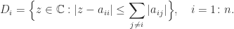
  lies in the union of the
 is nonnegative and
  , so
, so  converge as
  ? The answer is that it does, and the limit is stochastic, as long as
 , all even powers are equal to
  and all odd powers are equal to
  for all
  as
as  converges to the matrix with
  element is the probability of moving from state
  over a time step. It has nonnegative entries and the rows sum to
  , is a transition matrix for a time period a factor
  (years to months) and
  (weeks to days) are among the values of interest. Unfortunately, a stochastic

 (so that
  is row-stochastic). A matrix that is both row-stochastic and column-stochastic is called doubly stochastic. A permutation matrix is an example of a doubly stochastic matrix. If
  is a unitary matrix then the matrix with
  is doubly stochastic. A magic square scaled by the magic sum is also doubly stochastic. For example,
 , where
  is the number of positive eigenvalues of
  is the number of negative eigenvalues of
  is the number of zero eigenvalues of
  . The difference
  is called the signature.
 and
and  . But in general the diagonal elements do not tell us much about the inertia. For example, here is a matrix that has positive diagonal elements but only one positive eigenvalue (and this example works for any
  for a nonsingular matrix
  is nonsingular then
  .
. , and
, and  can be read off the diagonal of
  factorization, in which
  .
. and
and 
 .
.
 . From the
  we have

 it follows that
  .
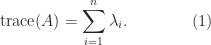
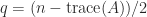
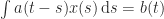
. are defined in terms of a summation over the rows of
  matrix
![\notag \left[\begin{array}{ccccc} 5/4 & 1 & 3/4 & 1/2 & 1/4 \\ 1 & 0 & 0 & 0 & 0\\ -1 & 1 & 0 & 0 & 0\\ 0 & 0 & 1 & 3 & 0\\ 0 & 0 & 0 & 1/2 & 5 \end{array}\right]](https://s0.wp.com/latex.php?latex=%5Cnotag+%5Cleft%5B%5Cbegin%7Barray%7D%7Bccccc%7D+5%2F4+++++++++%26+1+%26+3%2F4+++++++++%26+1%2F2+++++++++%26+1%2F4++++++++%5C%5C+1+%26+0+%26+0+%26+0+%26+0%5C%5C+-1+%26+1+%26+0+%26+0+%26+0%5C%5C+0+%26+0+%26+1+%26+3+%26+0%5C%5C+0+%26+0+%26+0+%26+1%2F2+++++++++%26+5+%5Cend%7Barray%7D%5Cright%5D+&bg=ffffff&fg=222222&s=0&c=20201002)
 The eigenvalues—three real and one complex conjugate pair—are the black dots. It happens that each disc contains an eigenvalue, but this is not always the case. For the matrix
![\notag \left[\begin{array}{cc} 2 & -1\\ 2 & 0 \end{array}\right]](https://s0.wp.com/latex.php?latex=%5Cnotag+%5Cleft%5B%5Cbegin%7Barray%7D%7Bcc%7D+2+%26+-1%5C%5C+2+%26+0+%5Cend%7Barray%7D%5Cright%5D+&bg=ffffff&fg=222222&s=0&c=20201002)
 and the blue disc does not contain an eigenvalue. The next result, which is proved by a continuity argument, provides additional information that increases the utility of Gershgorin’s theorem. In particular it says that if a disc is disjoint from the other discs then it contains an eigenvalue.
 would also lie in the disc, contradicting Theorem 2.
 for some nonsingular diagonal matrix
  . For
. For  the rightmost disc shrinks and remains distinct from the others and we obtain the sharper bounds
 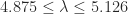 . The discs for
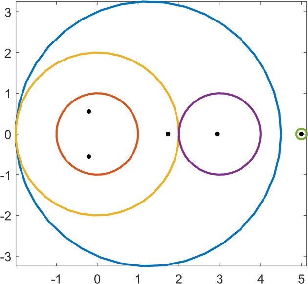
 for some positive integer
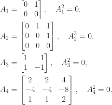
 is the
  matrix
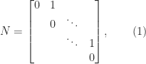

 . The superdiagonal of ones moves up to the right with each increase in the index of the power until it disappears off the top right corner of the matrix.
 has rank
  with
with  then
then  . We simply took orthogonal vectors
 ![x =[2, -4, 1]^T](https://s0.wp.com/latex.php?latex=x+%3D%5B2%2C+-4%2C+1%5D%5ET&bg=ffffff&fg=222222&s=0&c=20201002) and
and ![y = [1, 1, 2]^T](https://s0.wp.com/latex.php?latex=y+%3D+%5B1%2C+1%2C+2%5D%5ET&bg=ffffff&fg=222222&s=0&c=20201002) .
. with
with  implies
 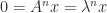 or
or  . Consequently, the trace and determinant of a nilpotent matrix are both zero.
 , since such a matrix has a spectral decomposition
  and the matrix
  is zero. It is only for nonnormal matrices that nilpotency is a nontrivial property, and the best way to understand it is with the Jordan canonical form (JCF). The JCF of a matrix with only zero eigenvalues has the form
  , where
  , where
  is of the form (1) and hence
  . It follows that the index of nilpotency is
  .
. and all other blocks are
  for
for  in (1).
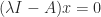 , which means that
  is singular, since
  . But
. But
 , the eigenvalues of
  , so if
  .
.
 are upper triangular, that is,
  for
for  . For such a matrix the eigenvalues are the diagonal elements.
 ) or Hermitian matrix (
 , where
  ) has real eigenvalues. A proof is
  so premultiplying the first equation by
  and postmultiplying the second by
  and
and  , which means that
  , or
, or  since
since  . The matrix
  ) or skew-Hermitian complex matrix (
 ) has pure imaginary eigenvalues. A proof is similar to the Hermitian case:
  and so
  is equal to both
  and
and  , so
, so  . The matrix
  above is skew-symmetric.
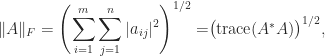
 , because for any matrix norm
  it can be shown that every eigenvalue satisfies
  .
.
 for some nonsingular matrix
  the matrix of eigenvalues. If we write
 ![X = [x_1,x_2,\dots,x_n]](https://s0.wp.com/latex.php?latex=X+%3D+%5Bx_1%2Cx_2%2C%5Cdots%2Cx_n%5D&bg=ffffff&fg=222222&s=0&c=20201002) then
then  ,
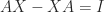
, ![\left[\begin{smallmatrix}1 \\ 0 \end{smallmatrix}\right]](https://s0.wp.com/latex.php?latex=%5Cleft%5B%5Cbegin%7Bsmallmatrix%7D1+%5C%5C+0+%5Cend%7Bsmallmatrix%7D%5Cright%5D&bg=ffffff&fg=222222&s=0&c=20201002) (or any nonzero scalar multiple of it). This matrix is a Jordan block. The matrix
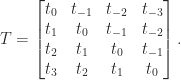
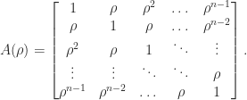
(or any nonzero scalar multiple of it). This matrix is a Jordan block. The matrix  is a Toeplitz matrix if
  for
for  parameters
  . A Toeplitz matrix has constant diagonals. For
  :
:
 .
. can be solved in less than the
  flops that would be required by LU factorization. Indeed methods are available that require only
  flops; see Golub and Van Loan (2013) for details.
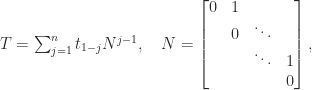
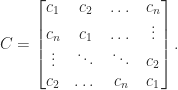
 . It follows that the product of two upper triangular Toeplitz matrices is again upper triangular Toeplitz, upper triangular Toeplitz matrices commute, and
  is also an upper triangular Toeplitz matrix (assuming
  is nonzero, so that
  is nonsingular).
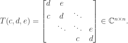
 are
are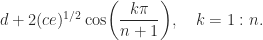
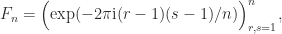
 , so that
  is a unitary matrix. (
 is a Vandermonde matrix with points the roots of unity.) Specifically,
 ). Moreover, the eigenvalues are given by
  , where
  is the first unit vector.
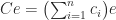 , where
  flops, since multiplication by
  , the
, the  version of which is
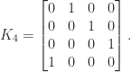

 . The eigenvalues are
  ,
,  , where
  . The matrix is singular when