The Cholesky factorization of a symmetric positive definite matrix 


As an example, the Cholesky factorization of the 


gallery('gcdmat',4) in MATLAB) is
![G_4 = \left[\begin{array}{cccc} 1 & 1 & 1 & 1\\ 1 & 2 & 1 & 2\\ 1 & 1 & 3 & 1\\ 1 & 2 & 1 & 4 \end{array}\right] = \left[\begin{array}{cccc} 1 & 0 & 0 & 0\\ 1 & 1 & 0 & 0\\ 1 & 0 & \sqrt{2} & 0\\ 1 & 1 & 0 & \sqrt{2} \end{array}\right] \left[\begin{array}{cccc} 1 & 1 & 1 & 1\\ 0 & 1 & 0 & 1\\ 0 & 0 & \sqrt{2} & 0\\ 0 & 0 & 0 & \sqrt{2} \end{array}\right].](https://s0.wp.com/latex.php?latex=G_4+%3D+%5Cleft%5B%5Cbegin%7Barray%7D%7Bcccc%7D+1+%26+1+%26+1+%26+1%5C%5C+1+%26+2+%26+1+%26+2%5C%5C+1+%26+1+%26+3+%26+1%5C%5C+1+%26+2+%26+1+%26+4+%5Cend%7Barray%7D%5Cright%5D+%3D+%5Cleft%5B%5Cbegin%7Barray%7D%7Bcccc%7D+1+%26+0+%26+0+%26+0%5C%5C+1+%26+1+%26+0+%26+0%5C%5C+1+%26+0+%26+%5Csqrt%7B2%7D+%26+0%5C%5C+1+%26+1+%26+0+%26+%5Csqrt%7B2%7D+%5Cend%7Barray%7D%5Cright%5D+%5Cleft%5B%5Cbegin%7Barray%7D%7Bcccc%7D+1+%26+1+%26+1+%26+1%5C%5C+0+%26+1+%26+0+%26+1%5C%5C+0+%26+0+%26+%5Csqrt%7B2%7D+%26+0%5C%5C+0+%26+0+%26+0+%26+%5Csqrt%7B2%7D+%5Cend%7Barray%7D%5Cright%5D.+&bg=ffffff&fg=222222&s=0&c=20201002)
The Cholesky factorization of an 


![\bigl[\begin{smallmatrix}1 & 1\\ 1& 2\end{smallmatrix}\bigr]= \bigl[\begin{smallmatrix}1 & 0\\ 1& 1\end{smallmatrix}\bigr] \bigl[\begin{smallmatrix}1 & 1\\ 0& 1\end{smallmatrix}\bigr]](https://s0.wp.com/latex.php?latex=%5Cbigl%5B%5Cbegin%7Bsmallmatrix%7D1+%26+1%5C%5C+1%26+2%5Cend%7Bsmallmatrix%7D%5Cbigr%5D%3D++%5Cbigl%5B%5Cbegin%7Bsmallmatrix%7D1+%26+0%5C%5C+1%26+1%5Cend%7Bsmallmatrix%7D%5Cbigr%5D++%5Cbigl%5B%5Cbegin%7Bsmallmatrix%7D1+%26+1%5C%5C+0%26+1%5Cend%7Bsmallmatrix%7D%5Cbigr%5D&bg=ffffff&fg=222222&s=0&c=20201002)
Inverting the Cholesky equation gives 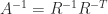


The Cholesky factorization is named after André-Louis Cholesky (1875–1918), a French military officer involved in geodesy and surveying in Crete and North Africa, who developed it for solving the normal equations arising in least squares problems.
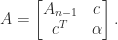
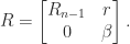
The existence and uniqueness of the factorization can be proved by induction on 

We know that 

Then
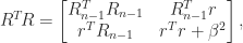
which equals

The first equation has a unique solution since 


we see that 

The quantity 

and since congruences preserve definiteness it follows that 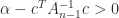
In textbooks it is common to see element-level equations for computing the Cholesky factorization, which come from directly solving the matrix equation 

What happens if this algorithm is executed on a general (indefinite) symmetric matrix that is, one that has both positive and negative eigenvalues? Line 5 will either attempt to take the square root of a negative number for some 


The MATLAB function chol normally returns an error message if the factorization fails. But a second output argument can be requested, which is set to the number of the stage on which the factorization failed, or to zero if the factorization succeeded. In the case of failure, the partially computed 

n = 8;
A = gallery('lehmer',n) - 0.3*eye(n); % Indefinite matrix.
[R,p] = chol(A)
z = [-R\(R'\A(1:p-1,p)); 1; zeros(n-p,1)];
neg_curve = z'*A*z
produces the output
R =
   8.3666e-01   5.9761e-01   3.9841e-01
            0   5.8554e-01   7.3193e-01
            0            0   7.4536e-02
p =
     4
neg_curve =
  -9.1437e+00
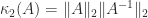
Cholesky factorization has excellent numerical stability. The computed factor 

where 


so the elements of
Once we have a Cholesky factorization we can use it to solve a linear system 


where 
Finally, what if 

![A = \left[\begin{array}{cccc} 1 & 1 & 1 & 1\\ 1 & 1 & 1 & 1\\ 1 & 1 & 2 & 2\\ 1 & 1 & 2 & 4\\ \end{array}\right] = \left[\begin{array}{cccc} 1 & 0 & 0 & 0\\ 1 & 0 & 0 & 0\\ 1 & 1 & 0 & 0\\ 1 & 1 & x & y\\ \end{array}\right] \left[\begin{array}{cccc} 1 & 1 & 1 & 1\\ 0 & 0 & 1 & 1\\ 0 & 0 & 0 & x\\ 0 & 0 & 0 & y\\ \end{array}\right] = R^T\!R](https://s0.wp.com/latex.php?latex=A+%3D+%5Cleft%5B%5Cbegin%7Barray%7D%7Bcccc%7D++1+%26+1+%26+1+%26+1%5C%5C++1+%26+1+%26+1+%26+1%5C%5C++1+%26+1+%26+2+%26+2%5C%5C++1+%26+1+%26+2+%26+4%5C%5C+%5Cend%7Barray%7D%5Cright%5D+%3D+%5Cleft%5B%5Cbegin%7Barray%7D%7Bcccc%7D+1+%26+0+%26+0+%26+0%5C%5C+1+%26+0+%26+0+%26+0%5C%5C+1+%26+1+%26+0+%26+0%5C%5C+1+%26+1+%26+x+%26+y%5C%5C+%5Cend%7Barray%7D%5Cright%5D+%5Cleft%5B%5Cbegin%7Barray%7D%7Bcccc%7D+1+%26+1+%26+1+%26+1%5C%5C+0+%26+0+%26+1+%26+1%5C%5C+0+%26+0+%26+0+%26+x%5C%5C+0+%26+0+%26+0+%26+y%5C%5C+%5Cend%7Barray%7D%5Cright%5D++%3D+R%5ET%5C%21R+&bg=ffffff&fg=222222&s=0&c=20201002)
for any 


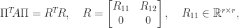
where 
![\Pi^T\mskip-5mu A\Pi = \left[\begin{array}{cccc} 4 & 2 & 1 & 1\\ 2 & 2 & 1 & 1\\ 1 & 1 & 1 & 1\\ 1 & 1 & 1 & 1 \end{array}\right] = \left[\begin{array}{cccc} 2 & 0 & 0 & 0\\ 1 & 1 & 0 & 0\\ \frac{1}{2} & \frac{1}{2} & \frac{\sqrt{2}}{2} & 0\\[2pt] \frac{1}{2} & \frac{1}{2} & \frac{\sqrt{2}}{2} & 0 \end{array}\right] \left[\begin{array}{cccc} 2 & 1 & \frac{1}{2} & \frac{1}{2}\\[2pt] 0 & 1 & \frac{1}{2} & \frac{1}{2}\\[2pt] 0 & 0 & \frac{\sqrt{2}}{2} & \frac{\sqrt{2}}{2}\\ 0 & 0 & 0 & 0 \end{array}\right],](https://s0.wp.com/latex.php?latex=%5CPi%5ET%5Cmskip-5mu+A%5CPi++%3D+%5Cleft%5B%5Cbegin%7Barray%7D%7Bcccc%7D+4+%26+2+%26+1+%26+1%5C%5C+2+%26+2+%26+1+%26+1%5C%5C+1+%26+1+%26+1+%26+1%5C%5C+1+%26+1+%26+1+%26+1+%5Cend%7Barray%7D%5Cright%5D++++%3D+%5Cleft%5B%5Cbegin%7Barray%7D%7Bcccc%7D+2+%26+0+%26+0+%26+0%5C%5C+1+%26+1+%26+0+%26+0%5C%5C+%5Cfrac%7B1%7D%7B2%7D+%26+%5Cfrac%7B1%7D%7B2%7D+%26+%5Cfrac%7B%5Csqrt%7B2%7D%7D%7B2%7D+%26+0%5C%5C%5B2pt%5D+%5Cfrac%7B1%7D%7B2%7D+%26+%5Cfrac%7B1%7D%7B2%7D+%26+%5Cfrac%7B%5Csqrt%7B2%7D%7D%7B2%7D+%26+0+%5Cend%7Barray%7D%5Cright%5D+%5Cleft%5B%5Cbegin%7Barray%7D%7Bcccc%7D+2+%26+1+%26+%5Cfrac%7B1%7D%7B2%7D+%26+%5Cfrac%7B1%7D%7B2%7D%5C%5C%5B2pt%5D+0+%26+1+%26+%5Cfrac%7B1%7D%7B2%7D+%26+%5Cfrac%7B1%7D%7B2%7D%5C%5C%5B2pt%5D+0+%26+0+%26+%5Cfrac%7B%5Csqrt%7B2%7D%7D%7B2%7D+%26+%5Cfrac%7B%5Csqrt%7B2%7D%7D%7B2%7D%5C%5C+0+%26+0+%26+0+%26+0+%5Cend%7Barray%7D%5Cright%5D%2C+&bg=ffffff&fg=222222&s=0&c=20201002)
which clearly displays the rank of
References
This is a minimal set of references, which contain further useful references within.
- Claude Brezinski, The Life and Work of André Cholesky, Numer. Algorithms 43, 279–288, 2006.
- Nicholas J. Higham, Cholesky factorization, WIREs Comp. Stat. 1(2), 251–254, 2009.
- Nicholas J. Higham, Accuracy and Stability of Numerical Algorithms, second edition, Society for Industrial and Applied Mathematics, Philadelphia, PA, USA, 2002. Chapter 10.
Related Blog Posts
This article is part of the “What Is” series, available from https://nhigham.com/category/what-is and in PDF form from the GitHub repository https://github.com/higham/what-is.
 of a scalar
  to
to  . The backward error of
 for a modest constant
  , where
  , where
 at
at  implies that a backward stable algorithm is automatically forward stable. The converse is not true. An example of an algorithm that is forward stable but not backward stable is Gauss–Jordan elimination for solving a linear system.
 small in the sense described above, then the algorithm for computing
 , where
  to satisfy
  for some small
  and
and  , meaning that
  matrix. But the computed
  independent rounding errors and is very unlikely to have rank
  , or both. For a nonlinear function we need to consider whether problem parameters are data; for example, for
  are the
  and the
  constants or are they data, like
  with
with  is a factorization
  , where
  has orthonormal columns and
  is Hermitian positive semidefinite. This decomposition is a generalization of the polar representation
  of a complex number, where
  corresponds to
  and
and  to
to  . When
  ,
,  , so
, so  , which is the unique positive semidefinite square root of
  . When
  is unique, and in this case
![A = \left[\begin{array}{@{}rr} 4 & 0\\ -5 & -3\\ 2 & 6 \end{array}\right] = \sqrt{2}\left[\begin{array}{@{}rr} \frac{1}{2} & -\frac{1}{6}\\[\smallskipamount] -\frac{1}{2} & -\frac{1}{6}\\[\smallskipamount] 0 & \frac{2}{3} \end{array}\right] \cdot \sqrt{2}\left[\begin{array}{@{\,}rr@{}} \frac{9}{2} & \frac{3}{2}\\[\smallskipamount] \frac{3}{2} & \frac{9}{2} \end{array}\right] \equiv UH.](https://s0.wp.com/latex.php?latex=A+%3D+%5Cleft%5B%5Cbegin%7Barray%7D%7B%40%7B%7Drr%7D+4+%26+0%5C%5C+-5+%26+-3%5C%5C+2+%26+6+%5Cend%7Barray%7D%5Cright%5D+++%3D+++%5Csqrt%7B2%7D%5Cleft%5B%5Cbegin%7Barray%7D%7B%40%7B%7Drr%7D+%5Cfrac%7B1%7D%7B2%7D+%26+-%5Cfrac%7B1%7D%7B6%7D%5C%5C%5B%5Csmallskipamount%5D+-%5Cfrac%7B1%7D%7B2%7D+%26+-%5Cfrac%7B1%7D%7B6%7D%5C%5C%5B%5Csmallskipamount%5D+0+%26+%5Cfrac%7B2%7D%7B3%7D+%5Cend%7Barray%7D%5Cright%5D+++%5Ccdot+++%5Csqrt%7B2%7D%5Cleft%5B%5Cbegin%7Barray%7D%7B%40%7B%5C%2C%7Drr%40%7B%7D%7D+%5Cfrac%7B9%7D%7B2%7D+%26+%5Cfrac%7B3%7D%7B2%7D%5C%5C%5B%5Csmallskipamount%5D+%5Cfrac%7B3%7D%7B2%7D+%26+%5Cfrac%7B9%7D%7B2%7D+%5Cend%7Barray%7D%5Cright%5D+++%5Cequiv+UH.+&bg=ffffff&fg=222222&s=0&c=20201002)
 and so
  . The equation

 and the norm is the Frobenius norm
 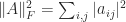 . This problem, which arises in factor analysis and in multidimensional scaling, asks how closely a unitary transformation of
  can reproduce
  , and there is a unique solution if
  and the polar decomposition can be computed by exploiting a relationship with quaternions.
 converge quadratically to
  is a singular value decomposition (SVD), where
  has orthonormal columns,
  is unitary, and
  is square and diagonal with nonnegative diagonal elements, then
 is a spectral decomposition (
 unitary,
  diagonal) then
  is an SVD. This latter relation is the basis of a method for computing the SVD that first computes the polar decomposition by a matrix iteration then computes the eigensystem of
  , are overcome in the canonical polar decomposition, defined for any
  and
and  . The superscript “
 ” denotes the Moore–Penrose pseudoinverse and a partial isometry can be characterized as a matrix
  .
. matrix
 ) and
) and

 for
for ![x = [1,{}-\!\sqrt{2},~1]^T](https://s0.wp.com/latex.php?latex=x+%3D+%5B1%2C%7B%7D-%5C%21%5Csqrt%7B2%7D%2C%7E1%5D%5ET&bg=ffffff&fg=222222&s=0&c=20201002) .
. for all
  .
. . Sometimes this condition can be confirmed from the definition of
  and
and  for
for  . Generally, though, this condition is not easy to check.
 , where the submatrix
  comprises the intersection of rows and columns
  , which also follows from the second condition since the determinant is the product of the eigenvalues.
 , where a square root is a matrix
  .
.![H_4 = \left[\begin{array}{@{\mskip 5mu}c*{3}{@{\mskip 15mu} c}@{\mskip 5mu}} 1 & \frac{1}{2} & \frac{1}{3} & \frac{1}{4} \\[6pt] \frac{1}{2} & \frac{1}{3} & \frac{1}{4} & \frac{1}{5}\\[6pt] \frac{1}{3} & \frac{1}{4} & \frac{1}{5} & \frac{1}{6}\\[6pt] \frac{1}{4} & \frac{1}{5} & \frac{1}{6} & \frac{1}{7}\\[6pt] \end{array}\right],](https://s0.wp.com/latex.php?latex=H_4+%3D+%5Cleft%5B%5Cbegin%7Barray%7D%7B%40%7B%5Cmskip+5mu%7Dc%2A%7B3%7D%7B%40%7B%5Cmskip+15mu%7D+c%7D%40%7B%5Cmskip+5mu%7D%7D+++++++++++++1+%26+%5Cfrac%7B1%7D%7B2%7D+%26+%5Cfrac%7B1%7D%7B3%7D++%26+%5Cfrac%7B1%7D%7B4%7D++%5C%5C%5B6pt%5D++++++++++++%5Cfrac%7B1%7D%7B2%7D+%26+%5Cfrac%7B1%7D%7B3%7D+++%26+%5Cfrac%7B1%7D%7B4%7D+++%26+%5Cfrac%7B1%7D%7B5%7D%5C%5C%5B6pt%5D++++++++++++%5Cfrac%7B1%7D%7B3%7D+%26+%5Cfrac%7B1%7D%7B4%7D+++%26++++++%5Cfrac%7B1%7D%7B5%7D+++%26+%5Cfrac%7B1%7D%7B6%7D%5C%5C%5B6pt%5D++++++++++++%5Cfrac%7B1%7D%7B4%7D+%26+%5Cfrac%7B1%7D%7B5%7D+++%26++++++%5Cfrac%7B1%7D%7B6%7D+++%26+%5Cfrac%7B1%7D%7B7%7D%5C%5C%5B6pt%5D++++++++++++%5Cend%7Barray%7D%5Cright%5D%2C+&bg=ffffff&fg=222222&s=0&c=20201002)
![P_4 = \left[\begin{array}{@{\mskip 5mu}c*{3}{@{\mskip 15mu} r}@{\mskip 5mu}} 1 & 1 & 1 & 1\\ 1 & 2 & 3 & 4\\ 1 & 3 & 6 & 10\\ 1 & 4 & 10 & 20 \end{array}\right],](https://s0.wp.com/latex.php?latex=P_4+%3D+%5Cleft%5B%5Cbegin%7Barray%7D%7B%40%7B%5Cmskip+5mu%7Dc%2A%7B3%7D%7B%40%7B%5Cmskip+15mu%7D+r%7D%40%7B%5Cmskip+5mu%7D%7D++++++1+%26++++1++%26+++1++%26+++1%5C%5C++++++1+%26++++2++%26+++3++%26+++4%5C%5C++++++1+%26++++3++%26+++6++%26++10%5C%5C++++++1+%26++++4++%26++10++%26++20++++++++++++%5Cend%7Barray%7D%5Cright%5D%2C+&bg=ffffff&fg=222222&s=0&c=20201002)
![S_4 = \left[\begin{array}{@{\mskip 5mu}c*{3}{@{\mskip 15mu} r}@{\mskip 5mu}} 2 & -1 & & \\ -1 & 2 & -1 & \\ & -1 & 2 & -1 \\ & & -1 & 2 \end{array}\right].](https://s0.wp.com/latex.php?latex=S_4+%3D+%5Cleft%5B%5Cbegin%7Barray%7D%7B%40%7B%5Cmskip+5mu%7Dc%2A%7B3%7D%7B%40%7B%5Cmskip+15mu%7D+r%7D%40%7B%5Cmskip+5mu%7D%7D++++++2+%26+++-1++%26++++++%26++++%5C%5C+++++-1+%26++++2++%26++-1++%26++++%5C%5C++++++++%26++++-1+%26+++2++%26++-1+%5C%5C++++++++%26+++++++%26++-1++%26++2++++++++++++%5Cend%7Barray%7D%5Cright%5D.+&bg=ffffff&fg=222222&s=0&c=20201002)
 is non-decreasing along the diagonals. However, if
  for any permutation matrix
  , so any symmetric reordering of the row or columns is possible without changing the definiteness.


 is congruent to a block diagonal matrix, which is positive definite when its diagonal blocks are. It follows that
  are positive definite. The matrix
  (Fischer’s inequality). Applying this inequality recursively gives Hadamard’s inequality for a symmetric positive definite
 for all
  , so that the quadratic form is allowed to be zero, then the symmetric matrix
  , being nonnegative; it is not enough to check the
 , and
, and  ) and
) and  for all nonzero vectors
  matrix to upper triangular form by elementary row operations. It consists of
  , where
  is unit lower triangular (lower triangular with ones on the diagonal) and
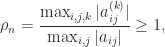
 are the elements at the start of the
  . Specifically, he obtained a bound for the backward error of the computed solution that is proportional to
  , where
  can be arbitrarily large, as is easily seen for
  . For some specific types of matrix more can be said.
 . In this case one would normally use Cholesky factorization instead of LU factorization.
 .
. .
. position at the start of stage
  and that equality is attained for matrices of the form illustrated for
  by
by![\left[\begin{array}{@{\mskip3mu}rrrr} 1 & 0 & 0 & 1 \\ -1 & 1 & 0 & 1 \\ -1 & -1 & 1 & 1 \\ -1 & -1 & -1 & 1 \\ \end{array} \right].](https://s0.wp.com/latex.php?latex=%5Cleft%5B%5Cbegin%7Barray%7D%7B%40%7B%5Cmskip3mu%7Drrrr%7D+++++++++++++++++++++++1++%26+0++%26+0++%26+1++%5C%5C+++++++++++++++++++++++-1+%26+1++%26+0++%26+1++%5C%5C+++++++++++++++++++++++-1+%26+-1+%26+1++%26+1++%5C%5C+++++++++++++++++++++++-1+%26+-1+%26+-1+%26+1++%5C%5C++++++++%5Cend%7Barray%7D++++++++%5Cright%5D.+&bg=ffffff&fg=222222&s=0&c=20201002)


 . Much interest has focused on the question of whether growth of
  , but such matrices do not exist for all
  and
and  .
. matrix with growth
  .
.
 is
is  , so it must be mapped back into
  be the given number and let
  and
and  with
with  be the adjacent numbers in
 and down to
  ; note that these probabilities sum to
 . In addition, certain results that hold for round to nearest, such as
  and
and  , can fail for stochastic rounding. What, then, is the benefit of stochastic rounding?
 , for example), so the expected error is zero. Hence stochastic rounding maintains, in a statistical sense, some of the information that is discarded by a deterministic rounding scheme. This property leads to some important benefits, as we now explain.
![[0,1]](https://s0.wp.com/latex.php?latex=%5B0%2C1%5D&bg=ffffff&fg=222222&s=0&c=20201002) then clearly the partial sum can grow monotonically as more and more terms are accumulated until at some point all the remaining terms “drop off the end” of the computed sum and do not change it—the sum stagnates. This phenomenon was observed and analyzed by Huskey and Hartree as long ago as 1949 in solving differential equations on the ENIAC. Stochastic rounding avoids stagnation by rounding up rather than down some of the time. The next figure gives an example. Here,
then clearly the partial sum can grow monotonically as more and more terms are accumulated until at some point all the remaining terms “drop off the end” of the computed sum and do not change it—the sum stagnates. This phenomenon was observed and analyzed by Huskey and Hartree as long ago as 1949 in solving differential equations on the ENIAC. Stochastic rounding avoids stagnation by rounding up rather than down some of the time. The next figure gives an example. Here,  ), and the backward errors are plotted for increasing
  , the errors for stochastic rounding (SR, in orange) are smaller than those for round to nearest (RTN, in blue), the latter quickly reaching 1.
 can be shown to hold with high probability. With round to nearest we have only the usual worst-case error bound, which is proportional to
  . In the figure above, the solid black line is the standard backward error bound
  is the
  . For example,
![H_4 = \left[\begin{array}{@{\mskip 5mu}c*{3}{@{\mskip 15mu} c}@{\mskip 5mu}} 1 & \frac{1}{2} & \frac{1}{3} & \frac{1}{4} \\[6pt] \frac{1}{2} & \frac{1}{3} & \frac{1}{4} & \frac{1}{5}\\[6pt] \frac{1}{3} & \frac{1}{4} & \frac{1}{5} & \frac{1}{6}\\[6pt] \frac{1}{4} & \frac{1}{5} & \frac{1}{6} & \frac{1}{7}\\[6pt] \end{array}\right].](https://s0.wp.com/latex.php?latex=H_4+%3D+%5Cleft%5B%5Cbegin%7Barray%7D%7B%40%7B%5Cmskip+5mu%7Dc%2A%7B3%7D%7B%40%7B%5Cmskip+15mu%7D+c%7D%40%7B%5Cmskip+5mu%7D%7D+++++++++++++1+%26+%5Cfrac%7B1%7D%7B2%7D+%26+%5Cfrac%7B1%7D%7B3%7D++%26+%5Cfrac%7B1%7D%7B4%7D++%5C%5C%5B6pt%5D++++++++++++%5Cfrac%7B1%7D%7B2%7D+%26+%5Cfrac%7B1%7D%7B3%7D+++%26+%5Cfrac%7B1%7D%7B4%7D+++%26+%5Cfrac%7B1%7D%7B5%7D%5C%5C%5B6pt%5D++++++++++++%5Cfrac%7B1%7D%7B3%7D+%26+%5Cfrac%7B1%7D%7B4%7D+++%26++++++%5Cfrac%7B1%7D%7B5%7D+++%26+%5Cfrac%7B1%7D%7B6%7D%5C%5C%5B6pt%5D++++++++++++%5Cfrac%7B1%7D%7B4%7D+%26+%5Cfrac%7B1%7D%7B5%7D+++%26++++++%5Cfrac%7B1%7D%7B6%7D+++%26+%5Cfrac%7B1%7D%7B7%7D%5C%5C%5B6pt%5D++++++++++++%5Cend%7Barray%7D%5Cright%5D.+&bg=ffffff&fg=222222&s=0&c=20201002)
 . An underlying reason for the ill conditioning is that the Hilbert matrix is obtained when least squares polynomial approximation is done using the monomial basis, and this is known to be an ill-conditioned polynomial basis.
 has integer entries, with
![H_4^{-1} = \left[\begin{array}{rrrr} 16 & -120 & 240 & -140 \\ -120 & 1200 & -2700 & 1680 \\ 240 & -2700 & 6480 & -4200 \\ -140 & 1680 & -4200 & 2800 \\ \end{array}\right].](https://s0.wp.com/latex.php?latex=H_4%5E%7B-1%7D+%3D+++++%5Cleft%5B%5Cbegin%7Barray%7D%7Brrrr%7D++++++16+%26+-120+%26+240+%26+-140+%5C%5C++++++-120+%26+1200+%26+-2700+%26+1680+%5C%5C++++++240+%26+-2700+%26+6480+%26+-4200+%5C%5C++++++-140+%26+1680+%26+-4200+%26+2800+%5C%5C++++++%5Cend%7Barray%7D%5Cright%5D.+&bg=ffffff&fg=222222&s=0&c=20201002)
 is positive semidefinite for all nonnegative real numbers
  .
. , which is a submatrix of
  , the largest singular value tends to
  as
as  , with error decaying slowly as
  , as was shown by Taussky.
 ), mean that certain quantities associated with it can be calculated more accurately than for a general positive definite matrix. The third reason why the Hilbert matrix is not a good test matrix is that most of its elements cannot be stored exactly in floating-point arithmetic, so the matrix actually stored is a perturbation of
  , but its elements are exactly representable in double precision only for
  .
. be Banach spaces (complete normed vector spaces). The Fréchet derivative of a function
  at
at  is a linear mapping
  such that
 . The notation
  should be read as “the Fréchet derivative of
  ”. The Fréchet derivative may not exist, but if it does exist then it is unique. When
  , the Fréchet derivative is just the usual derivative of a scalar function:
  .
. and
and  . From the expansion
 , the first order part of the expansion. If
  .
. with radius of convergence
  with
with  , the Fréchet derivative is
 , is
, is
 and
and  are Fréchet differentiable at
 given by

 is given in terms of the Fréchet derivative by

 are the divided differences
![\notag f[\lambda_i,\lambda_j] = \begin{cases} \dfrac{ f(\lambda_i)-f(\lambda_j) }{\lambda_i - \lambda_j}, & \lambda_i\ne\lambda_j, \\ f'(\lambda_i), & \lambda_i=\lambda_j, \end{cases}](https://s0.wp.com/latex.php?latex=%5Cnotag++++f%5B%5Clambda_i%2C%5Clambda_j%5D+%3D+%5Cbegin%7Bcases%7D++++%5Cdfrac%7B+f%28%5Clambda_i%29-f%28%5Clambda_j%29+%7D%7B%5Clambda_i+-+%5Clambda_j%7D%2C++++%26+%5Clambda_i%5Cne%5Clambda_j%2C+%5C%5C++++f%27%28%5Clambda_i%29%2C+%26+%5Clambda_i%3D%5Clambda_j%2C++++%5Cend%7Bcases%7D+&bg=ffffff&fg=222222&s=0&c=20201002)
 , where the
  are the eigenvalues of
  . Let
. Let  be an eigenpair of
  an eigenpair of
  , so that
  and
and  , and let
  . Then
 is an eigenvector of
  . But
. But ![f[\lambda,\mu] = (\lambda^2-\mu^2)/(\lambda - \mu) = \lambda + \mu](https://s0.wp.com/latex.php?latex=f%5B%5Clambda%2C%5Cmu%5D+%3D+%28%5Clambda%5E2-%5Cmu%5E2%29%2F%28%5Clambda+-+%5Cmu%29+%3D+%5Clambda+%2B+%5Cmu&bg=ffffff&fg=222222&s=0&c=20201002) (whether or not
(whether or not  and
and  are distinct).
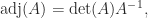
 denotes the submatrix of
  and column
  . It is the transposed matrix of cofactors. The adjugate is sometimes called the (classical) adjoint and is sometimes written as
  .
.
 and the fact that every matrix is the limit of a sequence of nonsingular matrices. Another property that can be proved in a similar way is
 or less then
  submatrix of
  in the definition of
  and
and  for any rank-1 matrix
 then
then  , then for nonsingular
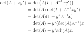


 be an SVD, where
  , with
  . Then
 is diagonal, with

 and so
 has modulus
  and
and  are the last columns of
  and
and  , so we must compute them. This function is numerically stable, as shown by Stewart (1998).
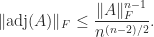

 , so
, so  is a square root of
  denotes the conjugate transpose).
 we have
 then we have
  , so that
  is a square root of
  .
. of a square matrix
  ,
, , where
  .
. satisfies all three conditions.)
 denotes the spectral radius. This definition is natural for functions that have a power series expansion, but it is rather limited in its applicability.
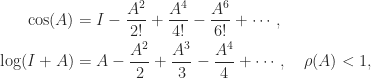


 has the derivatives of
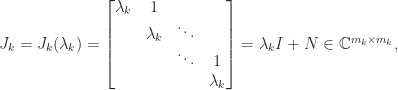
  , where
  is zero apart from a superdiagonal of 1s. The formula for
 : as
: as  we need the existence of the derivatives at
  with
with  then
then  .
. that encloses the spectrum of
