What Is the Sylvester Equation?

The Sylvester equation is the linear matrix equation

$AX - XB = C,$

where $A\in\mathbb{C}^{m\times m}$ , $B\in\mathbb{C}^{n\times n}$ , and $X,C\in\mathbb{C}^{m\times n}$ . It is named after James Joseph Sylvester (1814–1897), who considered the homogeneous version of the equation, $AX - XB = 0$ in 1884. Special cases of the equation are $Ax = b$ (a standard linear system), $AX = XA$ (matrix commutativity), $Ax = \lambda x$ (an eigenvalue–eigenvector equation), and $AX = I$ (matrix inversion).

In the case where $B = A$ , taking the trace of both sides of the equation gives

$\mathrm{trace}(C) = \mathrm{trace}(AX - XA) = \mathrm{trace}(AX) - \mathrm{trace} (XA) = 0,$

so a solution can exist only when $C$ has zero trace. Hence $AX - XA = I$ , for example, has no solution.

To determine when the Sylvester equation has a solution we will transform it into a simpler form. Let $A = URU^*$ and $B = VSV^*$ be Schur decompositions, where $U$ and $V$ are unitary and $R$ and $S$ are upper triangular. Premultiplying the Sylvester equation by $U^*$ , postmultiplying by $V$ , and setting $Y = U^*XV$ and $D = U^*CV$ , we obtain

$RY - YS = D,$

which is a Sylvester equation with upper triangular coefficient matrices. Equating the $j$ th columns on both sides leads to

$(R - s_{jj}I) y_j = d_j - \displaystyle\sum_{k=1}^{j-1} s_{kj} y_k, \quad j = 1\colon n.$

As long as the triangular matrices $R - s_{jj}I$ are nonsingular for all $j$ we can uniquely solve for $y_1$ , $y_2$ , …, $y_n$ in turn. Hence the Sylvester equation has a unique solution if $r_{ii} \ne s_{jj}$ for all $i$ and $j$ , that is, if $A$ and $B$ have no eigenvalue in common.

Since the Sylvester is a linear equation it must be possible to express it in the standard form “ $Ax = b$ ”. This can be done by applying the vec operator, which yields

$\qquad\qquad\qquad\qquad\qquad (I_n \otimes A - B^T \otimes I_m) \mathrm{vec}(X) = \mathrm{vec}(C), \qquad\qquad\qquad\qquad\qquad(*)$

where $\otimes$ is the Kronecker product. Using the Schur transformations above it is easy to show that the eigenvalues of the coefficient matrix are given in terms of those of $A$ and $B$ by

$\lambda_{ij} (I_n\otimes A - B^T\otimes I_m) = \lambda_i(A) - \lambda_j(B), \quad i=1\colon m, \quad j=1\colon n,$

so the coefficient matrix is nonsingular when $\lambda_i(A) \ne \lambda_j(B)$ for all $i$ and $j$ .

By considering the derivative of $Z(t) = \mathrm{e}^{At}C\mathrm{e}^{-Bt}$ , it can be shown that if the eigenvalues of $A$ and $-B$ have negative real parts (that is, $A$ and $-B$ are stable matrices) then

$X = -\displaystyle\int_0^{\infty} \mathrm{e}^{At} C \mathrm{e}^{-Bt} \, \mathrm{d}t$

is the unique solution of $AX - XB = C$ .

Applications

An important application of the Sylvester equation is in block diagonalization. Consider the block upper triangular matrix

$T = \begin{bmatrix} A & C\\ 0 & B \end{bmatrix}.$

If we can find a nonsingular matrix $Z$ such that $Z^{-1}TZ = \mathrm{diag}(A,B)$ then certain computations with $T$ become much easier. For example, for any function $f$ ,

$f(T) = f(Z \mathrm{diag}(A,B) Z^{-1}) = Zf(\mathrm{diag}(A,B)) Z^{-1} = Z\mathrm{diag}(f(A),f(B)) Z^{-1},$

so computing $f(T)$ reduces to computing $f(A)$ and $f(B)$ . Setting

$Z = \begin{bmatrix} I & -X\\ 0 & I \end{bmatrix}.$

and noting that $Z^{-1}$ is just $Z$ with the sign of the (1,2) block reversed, we find that

$Z^{-1} TZ = \begin{bmatrix} A & -AX + XB + C\\ 0 & B \end{bmatrix}.$

Hence $Z$ block diagonalizes $T$ if $X$ satisfies the Sylvester equation $AX - XB = C$ , which we know is possible if the eigenvalues of $A$ and $B$ are distinct. This restriction is unsurprising, as without it we could use this construction to diagonalize a $2\times 2$ Jordan block, which of course is impossible.

For another way in which Sylvester equations arises consider the expansion $(X+E)^2 = X^2 + XE + EX + E^2$ for square matrices $X$ and $E$ , from which it follows that $XE + EX$ is the Fréchet derivative of the function $x^2$ at $X$ in the direction $E$ , written $L_{x^2}(X,E)$ . Consequently, Newton’s method for the square root requires the solution of Sylvester equations, though in practice certain simplifications can be made to avoid their appearance. We can find the Fréchet derivative of $x^{1/2}$ by applying the chain rule to $\bigl(x^{1/2}\bigr)^2 = x$ , which gives $L_{x^2}\left(X^{1/2}, L_{x^{1/2}}(X,E)\right) = E$ . Therefore $Z = L_{x^{1/2}}(X,E)$ is the solution to the Sylvester equation $X^{1/2} Z + Z X^{1/2} = E$ . Consequently, the Sylvester equation plays a role in the perturbation theory for matrix square roots.

Sylvester equations also arise in the Schur–Parlett algorithm for computing matrix functions, which reduces a matrix to triangular Schur form $T$ and then solves $TF-FT = 0$ for $F = f(T)$ , blockwise, by a recurrence.

Solution Methods

How can we solve the Sylvester equation? One possibility is to solve $(*)$ by LU factorization with partial pivoting. However, the coefficient matrix is $mn\times mn$ and LU factorization cannot exploit the Kronecker product structure, so this approach is prohibitively expensive unless $m$ and $n$ are small. It is more efficient to compute Schur decompositions of $A$ and $B$ , transform the problem, and solve a sequence of triangular systems, as described above in our derivation of the conditions for the existence of a unique solution. This method was developed by Bartels and Stewart in 1972 and it is implemented in the MATLAB function sylvester.

In recent years research has focused particularly on solving Sylvester equations in which $A$ and $B$ are large and sparse and $C$ has low rank, which arise in applications in control theory and model reduction, for example. In this case it is usually possible to find good low rank approximations to $X$ and iterative methods based on Krylov subspaces have been very successful.

Sensitivity and the Separation

Define the separation of $A$ and $B$ by

$\mathrm{sep}(A,B) = \displaystyle\min_{Z\ne0} \displaystyle\frac{ \|AZ-ZB\|_F }{ \|Z\|_F }.$

The separation is positive if $A$ and $B$ have no eigenvalue in common, which we now assume. If $X$ is the solution to $AX - XB = C$ then

$\notag \mathrm{sep}(A,B) \le \displaystyle\frac{ \|AX-XB\|_F }{ \|X\|_F } = \frac{\|C\|_F}{\|X\|_F},$

so $X$ is bounded by

$\notag \|X\|_F \le \displaystyle\frac{\|C\|_F}{\mathrm{sep}(A,B)}.$

It is not hard to show that $\mathrm{sep}(A,B)^{-1} = \|P^{-1}\|_2$ , where $P$ is the matrix in $(*)$ . This bound on $\|X\|_F$ is a generalization of $\|x\|_2 \le \|A^{-1}\|_2 \|b\|_2$ for $Ax = b$ .

The separation features in a perturbation bound for the Sylvester equation. If

$\notag (A+\Delta A)(X+\Delta X) - (X+\Delta X)(B+\Delta B) = C+\Delta C,$

then

$\notag \displaystyle\frac{ \|\Delta X\|_F }{ \|X\|_F } \le 2\sqrt{3}\, \mathrm{sep}(A,B)^{-1} (\|A\|_F + \|B\|_F) \epsilon + O(\epsilon^2),$

where

$\notag \epsilon = \max \left\{ \displaystyle\frac{\|\Delta A\|_F}{\|A\|_F}, \frac{\|\Delta B\|_F}{\|B\|_F}, \frac{\|\Delta C\|_F}{\|C\|_F} \right\}.$

While we have the upper bound $\mathrm{sep}(A,B) \le \min_{i,j} |\lambda_i(A) - \lambda_j(B)|$ , this inequality can be extremely weak for nonnormal matrices, so two matrices can have a small separation even if their eigenvalues are well separated. To illustrate, let $T(\alpha)$ denote the $n\times n$ upper triangular matrix with $\alpha$ on the diagonal and $-1$ in all entries above the diagonal. The following table shows the values of $\mathrm{sep}(T(1),T(1.1))$ for several values of $n$ .

Even though the eigenvalues of $A$ and $B$ are $0.1$ apart, the separation is at the level of the unit roundoff for $n$ as small as $8$ .

The sep function was originally introduced by Stewart in the 1970s as a tool for studying the sensitivity of invariant subspaces.

Variations and Generalizations

The Sylvester equation has many variations and special cases, including the Lyapunov equation $AX + XA^* = C$ , the discrete Sylvester equation $X + AXB = C$ , and versions of all these for operators. It has also been generalized to multiple terms and to have coefficient matrices on both sides of $X$ , yielding

$\displaystyle\sum_{i=1}^k A_i X B_i = C.$

For $k\le 2$ and $m=n$ this equation can be solved in $O(n^3)$ flops. For $k > 2$ , no $O(n^3)$ flops algorithm is known and deriving efficient numerical methods remains an open problem. The equation arises in stochastic finite element discretizations of partial differential equations with random inputs, where the matrices $A_i$ and $B_i$ are large and sparse and, depending on the statistical properties of the random inputs, $k$ can be arbitrarily large.

References

This is a minimal set of references, which contain further useful references within.

Peter Lancaster, Explicit Solutions of Linear Matrix Equations, SIAM Review, 12(4), 544–566, 1970.
Nicholas J. Higham, Accuracy and Stability of Numerical Algorithms, second edition, Society for Industrial and Applied Mathematics, Philadelphia, PA, USA, 2002. Chapter 16.
Nicholas J. Higham, Functions of Matrices: Theory and Computation, Society for Industrial and Applied Mathematics, Philadelphia, PA, USA, 2008.
J. M. Varah, On the Separation of Two Matrices, SIAM J. Numer. Anal. 16 (2), 216–222, 1979.

What is the Kronecker Product?

The Kronecker product of two matrices $A\in\mathbb{C}^{m\times n}$ and $B\in\mathbb{C}^{p\times q}$ (also called the tensor product) is the $mp\times nq$ matrix¹

$A \otimes B = \begin{bmatrix} a_{11}B & a_{12}B & \dots & a_{1n}B \\ a_{21}B & a_{22}B & \dots & a_{2n}B \\ \vdots & \vdots & \ddots & \vdots \\ a_{m1}B & a_{m2}B & \dots & a_{mn}B \end{bmatrix}.$

In other words, $A\otimes B$ is the block $m\times n$ matrix with $(i,j)$ block $a_{ij}B$ . For example,

$\begin{bmatrix} a_{11} & a_{12} \\ a_{21} & a_{22} \end{bmatrix} \otimes \begin{bmatrix} b_{11} & b_{12} & b_{13} \\ b_{21} & b_{22} & b_{23} \end{bmatrix} = \left[\begin{array}{ccc|ccc} a_{11}b_{11} & a_{11}b_{12} & a_{11}b_{13} & a_{12}b_{11} & a_{12}b_{12} & a_{12}b_{13} \\ a_{11}b_{21} & a_{11}b_{22} & a_{11}b_{23} & a_{12}b_{21} & a_{12}b_{22} & a_{12}b_{23} \\\hline a_{21}b_{11} & a_{21}b_{12} & a_{21}b_{13} & a_{22}b_{11} & a_{22}b_{12} & a_{22}b_{13} \\ a_{21}b_{21} & a_{21}b_{22} & a_{21}b_{23} & a_{22}b_{21} & a_{22}b_{22} & a_{22}b_{23} \end{array}\right].$

Notice that the entries of $A\otimes B$ comprise every possible product $a_{ij}b_{rs}$ , which is not the case for the usual matrix product $AB$ when it is defined. Indeed if $A$ and $B$ are $n\times n$ then

$AB$ is $n\times n$ and contains sums of $n^3$ of the products $a_{ij}b_{rs}$ ,
$A\otimes B$ is $n^2\times n^2$ and contains all $n^4$ products $a_{ij}b_{rs}$ .

Two key properties of the Kronecker product are

$\begin{aligned} (A\otimes B)^* &= A^* \otimes B^*, \label{KP1} \\ (A\otimes B)(C\otimes D)&= AC \otimes BD. \label{KP2} \end{aligned}$

The second equality implies that when $x_i$ is an eigenvector of $A\in\mathbb{C}^{m\times m}$ with eigenvalue $\lambda_i$ and $y_j$ is an eigenvector of $B\in\mathbb{C}^{n\times n}$ with eigenvalue $\mu_j$ then

$(A\otimes B)(x_i\otimes y_j) = (Ax_i \otimes By_j) = (\lambda_i x_i \otimes \mu_j y_j) = \lambda_i\mu_j ( x_i \otimes y_j),$

so that $\lambda_i\mu_j$ is an eigenvalue of $A\otimes B$ with eigenvector $x_i \otimes y_j$ . In fact, the $mn$ eigenvalues of $A\otimes B$ are precisely $\lambda_i\mu_j$ for $i = 1\colon m$ and $j = 1\colon n$ .

Kronecker product structure arises in image deblurring models in which the blur is separable, that is, the blur in the horizontal direction can be separated from the blur in the vertical direction. Kronecker products also arise in the construction of Hadamard matrices. Recall that a Hadamard matrix is a matrix of $\pm1$ s whose rows and columns are mutually orthogonal. If $H_n$ is an $n\times n$ Hadamard matrix then

$\begin{bmatrix} \phantom{-} 1 & 1 \\ -1 & 1 \end{bmatrix} \otimes H_n = \begin{bmatrix} \phantom{-} H_n & H_n \\ -H_n & H_n \end{bmatrix}$

is a $2n\times 2n$ Hadamard matrix.

The practical significance of Kronecker product structure is that it allows computations on a large matrix to be reduced to computations on smaller matrices. For example, suppose $A$ and $B$ are Hermitian positive definite matrices and $C = A \otimes B$ , which can be shown to be Hermitian positive definite from the properties mentioned above. If $A = R^*R$ and $B = S^*S$ are Cholesky factorizations then

$A \otimes B = (R^*R) \otimes (S^*S) = (R^*\otimes S^*) (R \otimes S) = (R \otimes S)^* (R \otimes S),$

so $R\otimes S$ , which is easily seen to be triangular with positive diagonal elements, is the Cholesky factor of $A\otimes B$ . If $A$ and $B$ are $n\times n$ then forming $A\otimes B$ and computing its Cholesky factorization costs $O(n^6)$ flops, whereas $R$ and $S$ can be computed in $O(n^3)$ flops. If we want to solve a linear system $(A \otimes B)x = b$ this can be done using $R$ and $S$ without explicitly form $R\otimes S$ .

Vec Operator

The vec operator stacks the columns of a matrix into one long vector: if $A = [a_1,a_2,\dots,a_m]$ then $\mathrm{vec}(A) = [a_1^T a_2^T \dots a_m^T]^T$ . The vec operator and the Kronecker product interact nicely: for any $A$ , $X$ , and $B$ for which the product $AXB$ is defined,

$\mathrm{vec}(AXB) = (B^T \otimes A) \mathrm{vec}(X).$

This relation allows us to express a linear system $AXB = C$ in the usual form “ $Ax=b$ ”.

Kronecker Sum

The Kronecker sum of $A\in\mathbb{C}^{m\times m}$ and $B\in\mathbb{C}^{n\times n}$ is defined by $A\oplus B = A \otimes I_n + I_m \otimes B$ . The eigenvalues of $A\oplus B$ are $\lambda_{ij} = \lambda_i(A) + \lambda_j(B)$ , $i=1\colon m$ , $j=1\colon n$ , where the $\lambda_i(A)$ are the eigenvalues of $A$ and the $\lambda_j(B)$ are those of $B$ .

The Kronecker sum arises when we apply the vec operator to the matrix $AX + XB$ :

$\mathrm{vec}(AX + XB) = (I_m \otimes A + B^T \otimes I_n) \mathrm{vec}(X) = (B^T \oplus A) \mathrm{vec}(X).$

Kronecker sum structure also arises in finite difference discretizations of partial differential equations, such as when Poisson’s equation is discretized on a square by the usual five-point operator.

Vec-Permutation Matrix

Since for $A\in\mathbb{C}^{m\times n}$ the vectors $\mathrm{vec}(A)$ and $\mathrm{vec}(A^T)$ contain the same $mn$ elements in different orders, we must have

$\mathrm{vec}(A^T) = \Pi_{m,n} \mathrm{vec}(A),$

for some $mn\times mn$ permutation matrix $\Pi_{m,n}$ . This matrix is called the the vec-permutation matrix, and is also known as the commutation matrix.

Kronecker multiplication is not commutative, that is, $A \otimes B \ne B \otimes A$ in general, but $A \otimes B$ and $B \otimes A$ do contain the same elements in different orders. In fact, the two matrices are related by row and column permutations: if $A\in\mathbb{C}^{m\times n}$ and $B\in\mathbb{C}^{p\times q}$ then

$(A\otimes B)\Pi_{n,q} = \Pi_{m,p} (B\otimes A).$

This relation can be obtained as follows: for $X\in\mathbb{C}^{n\times q}$ ,

$\begin{aligned} (B \otimes A)\mathrm{vec}(X) &= \mathrm{vec}(AXB^T)\\ &= \Pi_{p,m} \mathrm{vec}(BX^TA^T)\\ &= \Pi_{p,m} (A\otimes B)\mathrm{vec}(X^T)\\ &= \Pi_{p,m} (A\otimes B) \Pi_{n,q}\mathrm{vec}(X). \end{aligned}$

Since these equalities hold for all $X$ , we have $B\otimes A = \Pi_{p,m} (A\otimes B) \Pi_{n,q}$ , from which the relation follows on using $\Pi_{m,n}\Pi_{n,m} = I$ , which can be obtained by replacing $A$ by $A^T$ in the definition of vec.

An explicit expression for the the vec-permutation matrix is

$\Pi_{m,n} = \displaystyle\sum_{i=1}^m \sum_{j=1}^n (e_i^{} e_j^T) \otimes (e_j^{} e_i^T),$

where $e_i$ is the $i$ th unit vector.

The following plot shows the sparsity patterns of all the vec permutation matrices $\Pi_{m,n}$ with $mn = 120$ , where the title of each subplot is $(m,n)$ .

MATLAB

In MATLAB the Kronecker product $A\otimes B$ can be computed as kron(A,B) and $\mathrm{vec}(A)$ is obtained by indexing with a colon: A(:). Be careful using kron as it can generate very large matrices!

Historical Note

The Kronecker product is named after Leopold Kronecker (1823–1891). Henderson et al. (1983) suggest that it should be called the Zehfuss product, after Johann Georg Zehfuss (1832–1891), who obtained the result $\det(A\otimes B) = \det(A)^n \det(B)^m$ for $A\in\mathbb{C}^{m\times m}$ and $B\in\mathbb{C}^{n\times n}$ in 1858.

References

This is a minimal set of references, which contain further useful references within.

Per Christian Hansen, James G. Nagy, and Dianne P. O’Leary, Deblurring Images: Matrices, Spectra, and Filtering, Society for Industrial and Applied Mathematics, Philadelphia, PA, USA, 2006.
Harold V. Henderson, Friedrich Pukelsheim, and Shayle R. Searle, On the History of the Kronecker Product, Linear and Multilinear Algebra 14(2), 113–120, 1983.
Harold V. Henderson and Shayle R. Searle, The Vec-Permutation Matrix, the Vec Operator and Kronecker Products: A Review, Linear and Multilinear Algebra 9, 271–288, 1981. Note: the definition of $\Pi_{m,n}$ gives the transpose of $\Pi_{m,n}$ as we have defined it.
Jan R. Magnus and Heinz Neudecker, The Commutation Matrix: Some Properties and Applications, Ann. Statist. 7, 381–394, 1979
Roger Horn and Charles Johnson, Topics in Matrix Analysis, Cambridge University Press, 1991. Chapter 4.
Charles F. Van Loan, The Ubiquitous Kronecker Product, J. Comput. Appl. Math. 123(1–2), 85–100, 2000.

Footnotes:

The $\otimes$ symbol is typed in $\LaTeX$ as \otimes.

What Is the Gerstenhaber Problem?

When Cayley introduced matrix algebra in 1858, he did much more than merely arrange numbers in a rectangular array. His definitions of addition, multiplication, and inversion produced an algebraic structure that has proved to be immensely useful, and which still holds many mysteries today.

An $n\times n$ matrix has $n^2$ parameters, so the vector space $\mathbb{R}^{n\times n}$ of real matrices has dimension $n^2$ , with a basis given by the matrices $E_{ij} = e_i^{}e_j^T$ , where $e_i$ is the vector that is zero except for a $1$ in the $i$ th entry. In his original paper, Cayley noticed the important property that the powers of a particular matrix $A$ can never span $\mathbb{R}^{n\times n}$ . The Cayley–Hamilton theorem says that $A$ satisfies its own characteristic equation, that is, $p(A) = 0$ where $p(t) = \det(t I - A)$ is the characteristic polynomial of $A$ . This means that $A^n$ can be expressed as a linear combination of $I$ , $A$ , …, $A^{n-1}$ , so the powers of $A$ span a vector space of dimension at most $n$ .

Gerstenhaber proved a generalization of this property in 1961: if $A$ and $B$ are two commuting $n\times n$ matrices then the matrices $A^iB^j$ , for all nonnegative $i$ and $j$ , generate a vector space of dimension at most $n$ . This result is much more difficult to prove than the Cayley–Hamilton theorem. Gerstenhaber’s proof was based on algebraic geometry, but purely matrix-theoretic proofs have been given.

A natural question, called the Gerstenhaber problem, is: does this result extend to three matrices, that is, does the vector space

$S_n = \{\, A^iB^jC^k: 0\le i,j,k \le n-1 \,\}$

have dimension at most $n$ for any $n\times n$ matrices $A$ , $B$ , and $C$ that commute with each other? (We can limit the powers to $n-1$ by the Cayley–Hamilton theorem.) The problem is defined over any field, but here I focus on the reals.

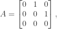
Before considering the three matrix case let us note that the answer is known to be “no” for four commuting $4\times 4$ matrices $A$ , $B$ , $C$ , and $D$ . Indeed let

$A = e_1^{}e_3^T, \quad B = e_1^{}e_4^T, \quad C = e_2^{}e_3^T, \quad D = e_2^{}e_4^T$

and note that all possible products of two of these matrices are zero, so the matrices commute pairwise. Yet $I = A^0, A, B, C, D$ are clearly five linearly independent matrices. Hence Gerstenhaber’s result does not extend to four matrices. It also does not extend to five or more matrices because it is known that the failure of the result for one value of $n$ implies failure for all larger $n$ . The question, then, is whether the three matrix case is like the two matrix case or the case for four or more matrices.

A great deal of effort has been put into proving or disproving the Gerstenhaber problem, so far without success. Here are two known facts.

The result holds for all $n\le 11$ .
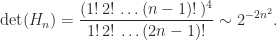
By a 1905 result of Schur, the dimension of $S_n$ is at most $1 + \lfloor n^2/4\rfloor$ , which is less than $n^2$ but still much bigger than $n$ . (Here, $\lfloor \cdot \rfloor$ is the floor function.)

One approach to investigating this problem is to look for a counterexample computationally. For some $n\ge 12$ , choose three commuting $n\times n$ matrices $A$ , $B$ , and $C$ , select $m\ge n$ monomials

$X_i = A^{i_p} B^{j_p} C^{k_p}, \quad 1\le p \le m,$

form the matrix

$Y = [\mathrm{vec}(X_1), \mathrm{vec}(X_2), \dots, \mathrm{vec}(X_m)],$

where $\mathrm{vec}$ converts a matrix into a vector by stacking the columns on top of each other, then compute $\mathrm{rank}(Y)$ , which is a lower bound on $\mathrm{dim}(S_n)$ , and check whether it is greater than $n$ .

This simple-minded approach has some obvious difficulties. How do we choose $A$ , $B$ , and $C$ ? How do we choose the powers? How do we avoid overflow and underflow and compute a reliable rank, given that we might be dealing with large powers of large matrices?

Holbrook and O’Meara (2020), who have written several papers on the Gerstenhaber problem, which they call the GP problem, state that they “firmly believe the GP will turn out to have a negative answer” and they have developed a sophisticated approach to searching for a case with $\mathrm{dim}(S_n) > n$ , which they call a “Eureka”. They first note that $A$ , $B$ and $C$ can be assumed to be nilpotent. This means that all three matrices must be defective, because a nondefective nilpotent matrix is zero. Next they note that since commuting matrices are simultaneously unitarily triangularizable, $A$ , $B$ , and $C$ can be assumed to be strictly upper triangular. Then they note that $A$ can be assumed to be in Weyr canonical form.

The Weyr canonical form is a dual of the Jordan canonical form in which the Jordan matrix is replaced by a Weyr matrix, which is a direct sum of basic Weyr matrices. A basic Weyr matrix has one distinct eigenvalue and is upper block bidiagonal with diagonal blocks that are multiples of the identity matrix and superdiagonal blocks that are rectangular identity matrices. The difference between Jordan and Weyr matrices is illustrated by the example

$J(\lambda) = \left[\begin{array}{ccc|cc} \lambda & 1 & 0 &&\\ 0 & \lambda & 1 &&\\ 0 & 0 & \lambda &&\\\hline & & &\lambda & 1\\ & & & 0 &\lambda \end{array}\right], \quad W(\lambda) = \left[\begin{array}{cc|cc|c} \lambda & 0 & 1 & 0&\\ 0 & \lambda & 0 & 1&\\\hline & & \lambda & 0 &1\\ & & 0 &\lambda & 0\\\hline & & & 0 &\lambda \end{array}\right],$

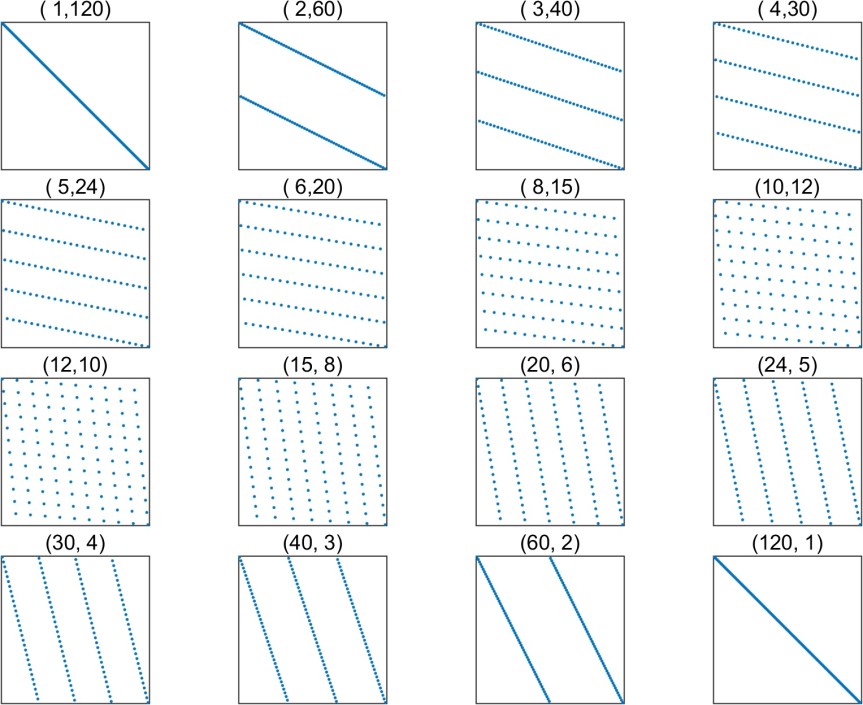
where the Jordan matrix $J(\lambda)$ and Weyr matrix $W(\lambda)$ are related by $J(\lambda) = P^TW(\lambda)P$ for some permutation matrix $P$ . There is an elegant way of relating the block sizes in the Jordan and Weyr matrices via a Young diagram. Form an array whose $k$ th column contains $j_k$ dots, where $j_k$ is the size of the $j$ th diagonal block of $J$ :

$\begin{array}{c|ccc} & j_1 & j_2\\\hline w_1 & \bullet & \bullet\\ w_2 & \bullet & \bullet\\ w_3 & \bullet & \end{array}$

Then the number of dots in the $k$ th row is the size of the $k$ th diagonal block in the Weyr form.

The reason for using the Weyr form is that whereas any matrix that commutes with a Jordan matrix has Toeplitz blocks, any matrix that commutes with a Weyr matrix is block upper triangular and is uniquely determined by the first block row. By choosing a Weyr form for $A$ , commuting matrices $B$ and $C$ can be built up in a systematic way.

Thanks to a result of O’Meara (2020) it suffices to compute modulo a prime $p$ , so the computations can be done in exact arithmetic, removing the need to worry about rounding errors or overflow.

Holbrook and O’Meara have mostly tried matrices up to dimension 50, but they feel that “the Loch Ness monster probably lives in deeper water, closer to $100\times 100$ ”. Their MATLAB codes (40 nicely commented but not optimized M-files) are available on request from the address given in their preprint. If you have the time to spare you might want to experiment with the codes and try to find a Eureka.

References

This is a minimal set of references, which contain further useful references within.

Robert M. Corless and Steven E. Thornton, The Weyr Canonical Form, 2016 (PDF poster).
John Holbrook and Kevin O’Meara, A Computing Strategy and Programs to Resolve the Gerstenhaber Problem for Commuting Triples of Matrices, ArXiv:2006.085882020, 2020.
John Holbrook and Kevin O’Meara, Commuting Triples of Matrices Vs the Computer, IMAGE (The Bulletin of the International Linear Algebra Society), to appear.
Kevin O’Meara, The Gerstenhaber Problem for Commuting Triples of Matrices is “Decidable”, Comm. Algebra 48, 453–466, 2020.
Kevin O’Meara, John Clark, and Charles Vinsonhaler, Advanced Topics in Linear Algebra. Weaving Matrix Problems Through the Weyr Form, Oxford University Press, Oxford, UK. 2011. Chapter 5.
B. A. Sethuraman, the Algebra Generated by Three Commuting Matrices, Math. Newsl. 21, 62–67, 2011.

This article is part of the “What Is” series, available from https://nhigham.com/category/what-is and in PDF form from the GitHub repository https://github.com/higham/what-is.

What Is a Cholesky Factorization?

The Cholesky factorization of a symmetric positive definite matrix $A$ is the factorization $A = R^T\!R$ , where $R$ is upper triangular with positive diagonal elements. It is a generalization of the property that a positive real number has a unique positive square root. The Cholesky factorization always exists and the requirement that the diagonal of $R$ be positive ensures that it is unique.

As an example, the Cholesky factorization of the $4\times 4$ matrix with $(i,j)$ element $\gcd(i,j)$ (gallery('gcdmat',4) in MATLAB) is

$G_4 = \left[\begin{array}{cccc} 1 & 1 & 1 & 1\\ 1 & 2 & 1 & 2\\ 1 & 1 & 3 & 1\\ 1 & 2 & 1 & 4 \end{array}\right] = \left[\begin{array}{cccc} 1 & 0 & 0 & 0\\ 1 & 1 & 0 & 0\\ 1 & 0 & \sqrt{2} & 0\\ 1 & 1 & 0 & \sqrt{2} \end{array}\right] \left[\begin{array}{cccc} 1 & 1 & 1 & 1\\ 0 & 1 & 0 & 1\\ 0 & 0 & \sqrt{2} & 0\\ 0 & 0 & 0 & \sqrt{2} \end{array}\right].$

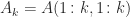The Cholesky factorization of an $n\times n$ matrix contains $n-1$ other Cholesky factorizations within it: $A_k = R_k^TR_k$ , $k=1:n-1$ , where $A_k = A(1\colon k,1\colon k)$ is the leading principal submatrix of order $k$ . For example, for $G_4$ with $k = 2$ , $\bigl[\begin{smallmatrix}1 & 1\\ 1& 2\end{smallmatrix}\bigr]= \bigl[\begin{smallmatrix}1 & 0\\ 1& 1\end{smallmatrix}\bigr] \bigl[\begin{smallmatrix}1 & 1\\ 0& 1\end{smallmatrix}\bigr]$ .

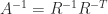
Inverting the Cholesky equation gives $A^{-1} = R^{-1} R^{-T}$ , which implies the interesting relation that the $(n,n)$ element of $A^{-1}$ is $r_{nn}^{-2}$ . So $G_4^{-1}$ has $(4,4)$ element $1/2$ . We also have $\det(A) = \det(R)^2 = (r_{11}\dots r_{nn})^2$ , so $\det(G_4) = 4$ for this matrix.

The Cholesky factorization is named after André-Louis Cholesky (1875–1918), a French military officer involved in geodesy and surveying in Crete and North Africa, who developed it for solving the normal equations arising in least squares problems.

The existence and uniqueness of the factorization can be proved by induction on $n$ , and the proof also serves as a method for computing it. Partition $A\in\mathbb{R}^{n\times n}$ as

$A = \begin{bmatrix} A_{n-1} & c \\ c^T & \alpha \end{bmatrix}.$

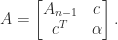
We know that $A_{n-1}$ is positive definite (any principal submatrix of a positive definite matrix is easily shown to be positive definite). Assume that $A_{n-1}$ has a unique Cholesky factorization $A_{n-1} = R_{n-1}^TR_{n-1}$ and define the upper triangular matrix

$R = \begin{bmatrix} R_{n-1} & r \\ 0 & \beta \end{bmatrix}.$

Then

$R^T\!R = \begin{bmatrix} R_{n-1}^T R_{n-1} & R_{n-1}^T r \\ r^T R_{n-1} & r^Tr + \beta^2 \end{bmatrix},$

which equals $A$ if and only if

$\begin{aligned} R_{n-1}^T r &= c, \\ r^Tr + \beta^2 &= \alpha. \end{aligned}$

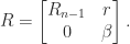
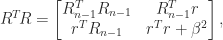
The first equation has a unique solution since $R_{n-1}$ is nonsingular. Then the second equation gives $\beta^2 = \alpha - r^Tr$ . It remains to check that there is a unique real, positive $\beta$ satisfying this equation. From the inequality

$0 < \det(A) = \det(R^T) \det(R) = \det(R_{n-1})^2 \beta^2$

we see that $\beta^2>0$ , hence there is a unique $\beta>0$ . This completes the inductive step.

The quantity $\alpha - r^Tr = \alpha - c^T A_{n-1}^{-1}c$ is the Schur complement of $A_{n-1}$ in $A$ . The essential reason why Cholesky factorization works is that the Schur complements of a positive definite matrix are themselves positive definite. Indeed we have the congruence

$\begin{bmatrix} I & 0 \\ -c^T A_{n-1}^{-1} & 1 \end{bmatrix} \begin{bmatrix} A_{n-1} & c \\ c^T & \alpha \end{bmatrix} \begin{bmatrix} I & -A_{n-1}^{-1}c\\ 0 & 1 \end{bmatrix} = \begin{bmatrix} A_{n-1} & 0 \\ 0 & \alpha - c^T A_{n-1}^{-1} c \end{bmatrix},$

and since congruences preserve definiteness it follows that $\alpha - c^T A_{n-1}^{-1} c > 0$ .

In textbooks it is common to see element-level equations for computing the Cholesky factorization, which come from directly solving the matrix equation $A = R^T\!R$ . If we equate elements on both sides, taking them a column at a time, starting with $a_{11} = r_{11}^2$ , then the following algorithm is obtained:

$\begin{array}{l} 1~ \mbox{for}~j=1:n \\ 2~ \quad \mbox{for}~ i=1:j-1 \\ 3~ \qquad r_{ij} = \bigl(a_{ij} - \sum_{k=1}^{i-1} r_{ki}r_{kj} \bigr) /r_{ii} \\ 4~ \quad \mbox{end} \\ 5~ \quad r_{jj} = \bigl(a_{jj} - \sum_{k=1}^{j-1} r_{kj}^2\bigr)^{1/2} \\ 6~ \mbox{end} \end{array}$

What happens if this algorithm is executed on a general (indefinite) symmetric matrix that is, one that has both positive and negative eigenvalues? Line 5 will either attempt to take the square root of a negative number for some $j$ or it will produce $r_{jj} = 0$ and on the next iteration of the loop we will have a division by zero. In floating-point arithmetic it is possible for the algorithm to fail for a positive definite matrix, but only if it is numerically singular: the algorithm is guaranteed to run to completion if the condition number $\kappa_2(A) = \|A\|_2 \|A^{-1}\|_2$ is safely less than $u^{-1}$ , where $u$ is the unit roundoff.

The MATLAB function chol normally returns an error message if the factorization fails. But a second output argument can be requested, which is set to the number of the stage on which the factorization failed, or to zero if the factorization succeeded. In the case of failure, the partially computed $R$ factor, returned in the first argument, can be used to compute a direction of negative curvature for $A$ , which is a vector $z$ such that $z^T\!Az < 0$ . Here is an example. The code

n = 8;
A = gallery('lehmer',n) - 0.3*eye(n); % Indefinite matrix.
[R,p] = chol(A)
z = [-R\(R'\A(1:p-1,p)); 1; zeros(n-p,1)];
neg_curve = z'*A*z

produces the output

R =
   8.3666e-01   5.9761e-01   3.9841e-01
            0   5.8554e-01   7.3193e-01
            0            0   7.4536e-02
p =
     4
neg_curve =
  -9.1437e+00

Cholesky factorization has excellent numerical stability. The computed factor $\widehat{R}$ satisfies

$A + \Delta A = \widehat{R}^T\widehat{R}, \quad \|\Delta A\|_2 \le c_nu\|A\|_2,$

where $c_n$ is a constant. Unlike for LU factorization there is no possibility of element growth; indeed for $i\le j$ ,

$r_{ij}^2 \le \displaystyle \sum_{k=1}^j r_{kj}^2 = a_{ij},$

so the elements of $R$ are nicely bounded relative to those of $A$ .

Once we have a Cholesky factorization we can use it to solve a linear system $Ax = b$ , by solving the lower triangular system $R^Ty = b$ and then the upper triangular system $Rx = y$ . The computed solution $\widehat{x}$ can be shown to satisfy

$(A+\Delta A)\widehat{x} = b, \quad \|\Delta A\|_2 \le d_nu\|A\|_2$

where $d_n$ is another constant. Thus $\widehat{x}$ has a small backward error.

Finally, what if $A$ is only symmetric positive semidefinite, that is, $x^T\!Ax \ge 0$ for all $x$ , so that $A$ is possibly singular? There always exists a Cholesky factorization (we can take the $R$ factor in the QR factorization of the positive semidefinite square root of $A$ ) but it may not be unique. For example, we have

$A = \left[\begin{array}{cccc} 1 & 1 & 1 & 1\\ 1 & 1 & 1 & 1\\ 1 & 1 & 2 & 2\\ 1 & 1 & 2 & 4\\ \end{array}\right] = \left[\begin{array}{cccc} 1 & 0 & 0 & 0\\ 1 & 0 & 0 & 0\\ 1 & 1 & 0 & 0\\ 1 & 1 & x & y\\ \end{array}\right] \left[\begin{array}{cccc} 1 & 1 & 1 & 1\\ 0 & 0 & 1 & 1\\ 0 & 0 & 0 & x\\ 0 & 0 & 0 & y\\ \end{array}\right] = R^T\!R$

for any $x$ and $y$ such that $x^2 + y^2 = 2$ . Note that $A$ has rank 3 but $R$ has two zero diagonal elements. When $A$ is positive semidefinite of rank $r$ what is usually wanted is a Cholesky factorization in which $R$ is zero in its last $n-r$ rows. Such a factorization can be obtained by using complete pivoting, which at each stage permutes the largest remaining diagonal element into the pivot position, which gives a factorization

$\Pi^T\mskip-5mu A\Pi = R^T\!R, \quad R = \begin{bmatrix} R_{11} & R_{12} \\ 0 & 0 \end{bmatrix}, \quad R_{11}\in\mathbb{R}^{r \times r},$

where $\Pi$ is a permutation matrix. For example, with $\Pi$ the identity matrix with its columns in reverse order,

$\Pi^T\mskip-5mu A\Pi = \left[\begin{array}{cccc} 4 & 2 & 1 & 1\\ 2 & 2 & 1 & 1\\ 1 & 1 & 1 & 1\\ 1 & 1 & 1 & 1 \end{array}\right] = \left[\begin{array}{cccc} 2 & 0 & 0 & 0\\ 1 & 1 & 0 & 0\\ \frac{1}{2} & \frac{1}{2} & \frac{\sqrt{2}}{2} & 0\\[2pt] \frac{1}{2} & \frac{1}{2} & \frac{\sqrt{2}}{2} & 0 \end{array}\right] \left[\begin{array}{cccc} 2 & 1 & \frac{1}{2} & \frac{1}{2}\\[2pt] 0 & 1 & \frac{1}{2} & \frac{1}{2}\\[2pt] 0 & 0 & \frac{\sqrt{2}}{2} & \frac{\sqrt{2}}{2}\\ 0 & 0 & 0 & 0 \end{array}\right],$

which clearly displays the rank of $A$ .

References

This is a minimal set of references, which contain further useful references within.

Claude Brezinski, The Life and Work of André Cholesky, Numer. Algorithms 43, 279–288, 2006.
Nicholas J. Higham, Cholesky factorization, WIREs Comp. Stat. 1(2), 251–254, 2009.
Nicholas J. Higham, Accuracy and Stability of Numerical Algorithms, second edition, Society for Industrial and Applied Mathematics, Philadelphia, PA, USA, 2002. Chapter 10.

What is Numerical Stability?

Numerical stability concerns how errors introduced during the execution of an algorithm affect the result. It is a property of an algorithm rather than the problem being solved. I will assume that the errors under consideration are rounding errors, but in principle the errors can be from any source.

Consider a scalar function $y = f(x)$ of a scalar $x$ . We regard $x$ as the input data and $y$ as the output. The forward error of a computed approximation $\widehat{y}$ to $y$ is the relative error $|y - \widehat{y}|/|y|$ . The backward error of $\widehat{y}$ is

$\min\left\{\, \displaystyle\frac{|\Delta x|}{|x|}: \widehat{y} = f(x+\Delta x) \,\right\}.$

If $\widehat{y}$ has a small backward error then it is the exact answer for a slightly perturbed input. Here, “small’ is interpreted relative to the floating-point arithmetic, so a small backward error means one of the form $cu$ for a modest constant $c$ , where $u$ is the unit roundoff.

An algorithm that always produces a small backward error is called backward stable. In a backward stable algorithm the errors introduced during the algorithm have the same effect as a small perturbation in the data. If the backward error is the same size as any uncertainty in the data then the algorithm produces as good a result as we can expect.

If $x$ undergoes a relative perturbation of size $u$ then $y = f(x)$ can change by as much as $\mathrm{cond}_f(x) u$ , where

$\mathrm{cond}_f(x) = \lim_{\epsilon\to0} \displaystyle\sup_{|\Delta x| \le \epsilon |x|} \displaystyle\frac{|f(x+\Delta x) - f(x)|}{\epsilon|f(x)|}$

is the condition number of $f$ at $x$ . An algorithm that always produces $\widehat{y}$ with a forward error of order $\mathrm{cond}_f(x) u$ is called forward stable.

The definition of $\mathrm{cond}_f(x)$ implies that a backward stable algorithm is automatically forward stable. The converse is not true. An example of an algorithm that is forward stable but not backward stable is Gauss–Jordan elimination for solving a linear system.

If $\widehat{y}$ satisfies

$\widehat{y} + \Delta y = f(x+\Delta x), \quad |\Delta y| \le \epsilon |\widehat{y}|, \quad |\Delta x| \le \epsilon |x|,$

with $\epsilon$ small in the sense described above, then the algorithm for computing $y$ is mixed backward–forward stable. Such an algorithm produces almost the right answer for a slightly perturbed input. The following diagram illustrates the previous equation.

With these definitions in hand, we can turn to the meaning of the term numerically stable. Depending on the context, numerical stability can mean that an algorithm is (a) backward stable, (b) forward stable, or (c) mixed backward–forward stable.

For some problems, backward stability is difficult or impossible to achieve, so numerical stability has meaning (b) or (c). For example, let $Z = xy^T$ , where $x$ and $y$ are $n$ -vectors. Backward stability would require the computed $\widehat{Z}$ to satisfy $\widehat{Z} = (x+\Delta x)(y+\Delta y)^T$ for some small $\Delta x$ and $\Delta y$ , meaning that $\widehat{Z}$ is a rank- $1$ matrix. But the computed $\widehat{Z}$ contains $n^2$ independent rounding errors and is very unlikely to have rank $1$ .

We briefly mention some other relevant points.

What is the data? For a linear system $Ax = b$ the data is $A$ or $b$ , or both. For a nonlinear function we need to consider whether problem parameters are data; for example, for $f(x) = \cos(3x^2+2)$ are the $3$ and the $2$ constants or are they data, like $x$ , that can be perturbed?
We have measured perturbations in a relative sense. Absolute errors can also be used.
For problems whose inputs are matrices or vectors we need to use norms or componentwise measures.
Some algorithms are only unconditionally numerically stable, that is, they are numerically stable for some subset of problems. For example, the normal equations method for solving a linear least squares problem is forward stable for problems with a large residual.

References

This is a minimal set of references, which contain further useful references within.

Robert M. Corless and Nicolas Fillion, A Graduate Introduction to Numerical Methods from the Viewpoint of Backward Error Analysis, Springer, New York, 2013. My review of this book.
Nicholas J. Higham, Accuracy and Stability of Numerical Algorithms, second edition, Society for Industrial and Applied Mathematics, Philadelphia, PA, USA, 2002.

What is the Polar Decomposition?

A polar decomposition of $A\in\mathbb{C}^{m \times n}$ with $m \ge n$ is a factorization $A = UH$ , where $U\in\mathbb{C}^{m \times n}$ has orthonormal columns and $H\in\mathbb{C}^{n \times n}$ is Hermitian positive semidefinite. This decomposition is a generalization of the polar representation $z = r \mathrm{e}^{\mathrm{i}\theta}$ of a complex number, where $H$ corresponds to $r\ge 0$ and $U$ to $\mathrm{e}^{\mathrm{i}\theta}$ . When $A$ is real, $H$ is symmetric positive semidefinite. When $m = n$ , $U$ is a square unitary matrix (orthogonal for real $A$ ).

We have $A^*A = H^*U^*UH = H^2$ , so $H = (A^*\!A)^{1/2}$ , which is the unique positive semidefinite square root of $A^*A$ . When $A$ has full rank, $H$ is nonsingular and $U = AH^{-1}$ is unique, and in this case $U$ can be expressed as

$U = \displaystyle\frac{2}{\pi} A \displaystyle\int_{0}^{\infty} (t^2I+A^*\!A)^{-1}\, \mathrm{d}t.$

An example of a polar decomposition is

$A = \left[\begin{array}{@{}rr} 4 & 0\\ -5 & -3\\ 2 & 6 \end{array}\right] = \sqrt{2}\left[\begin{array}{@{}rr} \frac{1}{2} & -\frac{1}{6}\\[\smallskipamount] -\frac{1}{2} & -\frac{1}{6}\\[\smallskipamount] 0 & \frac{2}{3} \end{array}\right] \cdot \sqrt{2}\left[\begin{array}{@{\,}rr@{}} \frac{9}{2} & \frac{3}{2}\\[\smallskipamount] \frac{3}{2} & \frac{9}{2} \end{array}\right] \equiv UH.$

For an example with a rank-deficient matrix consider

$A = \begin{bmatrix} 0 & 1 & 0 \\ 0 & 0 & 1 \\ 0 & 0 & 0 \end{bmatrix},$

for which $A^*A = \mathrm{diag}(0,1,1)$ and so $H = \mathrm{diag}(0,1,1)$ . The equation $A = UH$ then implies that

$U = \begin{bmatrix} 0 & 1 & 0 \\ 0 & 0 & 1 \\ \theta & 0 & 0 \end{bmatrix}, \quad |\theta| = 1,$

so $U$ is not unique.

The polar factor $U$ has the important property that it is a closest matrix with orthonormal columns to $A$ in any unitarily invariant norm. Hence the polar decomposition provides an optimal way to orthogonalize a matrix. This method of orthogonalization is used in various applications, including in quantum chemistry, where it is called Löwdin orthogonalization. Most often, though, orthogonalization is done through QR factorization, trading optimality for a faster computation.

An important application of the polar decomposition is to the orthogonal Procrustes problem¹

$\min \bigl\{\, \|A-BW\|_F: W \in \mathbb{C}^{n\times n},\; W^*W = I \,\bigr\},$

where $A,B\in\mathbb{C}^{m\times n}$ and the norm is the Frobenius norm $\|A\|_F^2 = \sum_{i,j} |a_{ij}|^2$ . This problem, which arises in factor analysis and in multidimensional scaling, asks how closely a unitary transformation of $B$ can reproduce $A$ . Any solution is a unitary polar factor of $B^*\!A$ , and there is a unique solution if $B^*\!A$ is nonsingular. Another application of the polar decomposition is in 3D graphics transformations. Here, the matrices are $3\times 3$ and the polar decomposition can be computed by exploiting a relationship with quaternions.

For a square nonsingular matrix $A$ , the unitary polar factor $U$ can be computed by a Newton iteration:

$X_{k+1} = \displaystyle\frac{1}{2} (X_k + X_k^{-*}), \quad X_0 = A.$

The iterates $X_k$ converge quadratically to $U$ . This is just one of many iterations for computing $U$ and much work has been done on the efficient implementation of these iterations.

If $A = P \Sigma Q^*$ is a singular value decomposition (SVD), where $P\in\mathbb{C}^{m\times n}$ has orthonormal columns, $Q\in\mathbb{C}^{n\times n}$ is unitary, and $\Sigma$ is square and diagonal with nonnegative diagonal elements, then

$A = PQ^* \cdot Q \Sigma Q^* \equiv UH,$

where $U$ has orthonormal columns and $H$ is Hermitian positive semidefinite. So a polar decomposition can be constructed from an SVD. The converse is true: if $A = UH$ is a polar decomposition and $H = Q\Sigma Q^*$ is a spectral decomposition ( $Q$ unitary, $D$ diagonal) then $A = (UQ)\Sigma Q^* \equiv P \Sigma Q^*$ is an SVD. This latter relation is the basis of a method for computing the SVD that first computes the polar decomposition by a matrix iteration then computes the eigensystem of $H$ , and which is extremely fast on distributed-memory manycore computers.

The nonuniqueness of the polar decomposition for rank deficient $A$ , and the lack of a satisfactory definition of a polar decomposition for $m < n$ , are overcome in the canonical polar decomposition, defined for any $m$ and $n$ . Here, $A = UH$ with $U$ a partial isometry, $H$ is Hermitian positive semidefinite, and $U^*U = HH^+$ . The superscript “ $+$ ” denotes the Moore–Penrose pseudoinverse and a partial isometry can be characterized as a matrix $U$ for which $U^+ = U^*$ .

Generalizations of the (canonical) polar decomposition have been investigated in which the properties of $U$ and $H$ are defined with respect to a general, possibly indefinite, scalar product.

References

This is a minimal set of references, which contain further useful references within.

Nicholas J. Higham, Functions of Matrices: Theory and Computation, Society for Industrial and Applied Mathematics, Philadelphia, PA, USA, 2008. (Chapter 8.)
Nicholas Higham, Christian Mehl, and Françoise Tisseur, The canonical generalized polar decomposition, SIAM J. Matrix Anal. Appl. 31(4), 2163–2180, 2010.
Nicholas J. Higham and Vanni Noferini, An algorithm to compute the polar decomposition of a $3 \times 3$ matrix, Numer. Algorithms 73, 349–369, 2016.
Yuji Nakatsukasa and Nicholas J. Higham, Stable and efficient spectral divide and conquer algorithms for the symmetric eigenvalue decomposition and the SVD, SIAM J. Sci. Comput. 35(3), A1325–A1349, 2013.
Dalal Sukkari, Hatem Ltaief, Aniello Esposito, and David Keyes, A QDWH-based SVD software framework on distributed-memory manycore systems, ACM Trans. Math. Software 45, 18:1–18:21, 2019.

Footnotes:

Procrustes: an ancient Greek robber who tied his victims to an iron bed, stretching their legs if too short for it, and lopping them if too long.

What Is a Symmetric Positive Definite Matrix?

A real $n\times n$ matrix $A$ is symmetric positive definite if it is symmetric ( $A$ is equal to its transpose, $A^T$ ) and

$x^T\!Ax > 0 \quad \mbox{for all nonzero vectors}~x.$

By making particular choices of $x$ in this definition we can derive the inequalities

$\begin{alignedat}{2} a_{ii} &>0 \quad&&\mbox{for all}~i,\\ a_{ij} &< \sqrt{ a_{ii} a_{jj} } \quad&&\mbox{for all}~i\ne j. \end{alignedat}$

Satisfying these inequalities is not sufficient for positive definiteness. For example, the matrix

$A = \begin{bmatrix} 1 & 3/4 & 0 \\ 3/4 & 1 & 3/4 \\ 0 & 3/4 & 1 \\ \end{bmatrix}$

satisfies all the inequalities but $x^T\!Ax < 0$ for $x = [1,{}-\!\sqrt{2},~1]^T$ .

A sufficient condition for a symmetric matrix to be positive definite is that it has positive diagonal elements and is diagonally dominant, that is, $a_{ii} > \sum_{j \ne i} |a_{ij}|$ for all $i$ .

The definition requires the positivity of the quadratic form $x^T\!Ax$ . Sometimes this condition can be confirmed from the definition of $A$ . For example, if $A = B^T\!B$ and $B$ has linearly independent columns then $x^T\!Ax = (Bx)^T Bx > 0$ for $x\ne 0$ . Generally, though, this condition is not easy to check.

Two equivalent conditions to $A$ being symmetric positive definite are

every leading principal minor $\det(A_k)$ , where the submatrix $A_k = A(1\colon k, 1 \colon k)$ comprises the intersection of rows and columns $1$ to $k$ , is positive,
the eigenvalues of $A$ are all positive.

The first condition implies, in particular, that $\det(A) > 0$ , which also follows from the second condition since the determinant is the product of the eigenvalues.

Here are some other important properties of symmetric positive definite matrices.

$A^{-1}$ is positive definite.
$A$ has a unique symmetric positive definite square root $X$ , where a square root is a matrix $X$ such that $X^2 = A$ .
$A$ has a unique Cholesky factorization $A = R^T\!R$ , where $R$ is upper triangular with positive diagonal elements.

Sources of positive definite matrices include statistics, since nonsingular correlation matrices and covariance matrices are symmetric positive definite, and finite element and finite difference discretizations of differential equations.

Examples of symmetric positive definite matrices, of which we display only the $4\times 4$ instances, are the Hilbert matrix

$H_4 = \left[\begin{array}{@{\mskip 5mu}c*{3}{@{\mskip 15mu} c}@{\mskip 5mu}} 1 & \frac{1}{2} & \frac{1}{3} & \frac{1}{4} \\[6pt] \frac{1}{2} & \frac{1}{3} & \frac{1}{4} & \frac{1}{5}\\[6pt] \frac{1}{3} & \frac{1}{4} & \frac{1}{5} & \frac{1}{6}\\[6pt] \frac{1}{4} & \frac{1}{5} & \frac{1}{6} & \frac{1}{7}\\[6pt] \end{array}\right],$

the Pascal matrix

$P_4 = \left[\begin{array}{@{\mskip 5mu}c*{3}{@{\mskip 15mu} r}@{\mskip 5mu}} 1 & 1 & 1 & 1\\ 1 & 2 & 3 & 4\\ 1 & 3 & 6 & 10\\ 1 & 4 & 10 & 20 \end{array}\right],$

and minus the second difference matrix, which is the tridiagonal matrix

$S_4 = \left[\begin{array}{@{\mskip 5mu}c*{3}{@{\mskip 15mu} r}@{\mskip 5mu}} 2 & -1 & & \\ -1 & 2 & -1 & \\ & -1 & 2 & -1 \\ & & -1 & 2 \end{array}\right].$

All three of these matrices have the property that $a_{ij}$ is non-decreasing along the diagonals. However, if $A$ is positive definite then so is $P^TAP$ for any permutation matrix $P$ , so any symmetric reordering of the row or columns is possible without changing the definiteness.

A $4\times 4$ symmetric positive definite matrix that was often used as a test matrix in the early days of digital computing is the Wilson matrix

$W = \begin{bmatrix} 5 &7& 6& 5 \\ 7 &10& 8& 7 \\ 6& 8& 10& 9 \\ 5& 7& 9 &10 \end{bmatrix}.$

What is the best way to test numerically whether a symmetric matrix is positive definite? Computing the eigenvalues and checking their positivity is reliable, but slow. The fastest method is to attempt to compute a Cholesky factorization and declare the matrix positivite definite if the factorization succeeds. This is a reliable test even in floating-point arithmetic. If the matrix is not positive definite the factorization typically breaks down in the early stages so and gives a quick negative answer.

Symmetric block matrices

$C = \begin{bmatrix} A & X\\ X^T & B \end{bmatrix}$

often appear in applications. If $A$ is nonsingular then we can write

$\begin{bmatrix} A & X\\ X^T & B \end{bmatrix} = \begin{bmatrix} I & 0\\ X^TA^{-1} & I \end{bmatrix} \begin{bmatrix} A & 0\\ 0 & B-X^TA^{-1}X \end{bmatrix} \begin{bmatrix} I & A^{-1}X\\ 0 & I \end{bmatrix},$

which shows that $C$ is congruent to a block diagonal matrix, which is positive definite when its diagonal blocks are. It follows that $C$ is positive definite if and only if both $A$ and $B - X^TA^{-1}X$ are positive definite. The matrix $B - X^TA^{-1}X$ is called the Schur complement of $A$ in $C$ .

We mention two determinantal inequalities. If the block matrix $C$ above is positive definite then $\det(C) \le \det(A) \det(B)$ (Fischer’s inequality). Applying this inequality recursively gives Hadamard’s inequality for a symmetric positive definite $A$ :

$\det(A) \le a_{11}a_{22} \dots a_{nn},$

with equality if and only if $A$ is diagonal.

Finally, we note that if $x^TAx \ge 0$ for all $x\ne0$ , so that the quadratic form is allowed to be zero, then the symmetric matrix $A$ is called symmetric positive semidefinite. Some, but not all, of the properties above generalize in a natural way. An important difference is that semidefinitness is equivalent to all principal minors, of which there are $2^{n-1}$ , being nonnegative; it is not enough to check the $n$ leading principal minors. Consider, as an example, the matrix

$\begin{bmatrix} 1 & 1 & 1\\ 1 & 1 & 1\\ 1 & 1 & 0 \end{bmatrix},$

which has leading principal minors $1$ , $0$ , and $0$ and a negative eigenvalue.

A complex $n\times n$ matrix $A$ is Hermitian positive definite if it is Hermitian ( $A$ is equal to its conjugate transpose, $A^*$ ) and $x^*Ax > 0$ for all nonzero vectors $x$ . Everything we have said above generalizes to the complex case.

References

This is a minimal set of references, which contain further useful references within.

Rajendra Bhatia, Positive Definite Matrices, Princeton University Press, Princeton, NJ, USA, 2007.
Nicholas J. Higham, Computing a nearest symmetric positive semidefinite matrix, Linear Algebra Appl. 103, 103–118, 1988. Section 5.
Roger A. Horn and Charles R. Johnson, Matrix Analysis, second edition, Cambridge University Press, 2013. My review of the second edition.

What Is the Growth Factor for Gaussian Elimination?

Gaussian elimination is the process of reducing an $n \times n$ matrix to upper triangular form by elementary row operations. It consists of $n$ stages, in the $k$ th of which multiples of row $k$ are added to later rows to eliminate elements below the diagonal in the $k$ th column. The result of Gaussian elimination (assuming it succeeds) is a factorization $A = LU$ , where $L$ is unit lower triangular (lower triangular with ones on the diagonal) and $U$ is upper triangular. This factorization reduces the solution of a linear system $Ax = b$ to the solution of two triangular systems.

James Wilkinson showed in the early 1960s that the numerical stability of Gaussian elimination depends on the growth factor

$\rho_n = \displaystyle\frac{\max_{i,j,k} |a_{ij}^{(k)}|} {\max_{i,j}|a_{ij}|} \ge 1,$

where the $a_{ij}^{(k)}$ are the elements at the start of the $k$ th stage of Gaussian elimination, with $A = \bigl(a_{ij}^{(1)}\bigr)$ . Specifically, he obtained a bound for the backward error of the computed solution that is proportional to $\rho_nu$ , where $u$ is the unit roundoff of the floating-point arithmetic. Wilkinson’s analysis focused attention on the size of the growth factor.

If no row interchanges are done during the elimination then $\rho_n$ can be arbitrarily large, as is easily seen for $n = 2$ . For some specific types of matrix more can be said.

If $A$ is symmetric positive definite then $\rho_n = 1$ . In this case one would normally use Cholesky factorization instead of LU factorization.
If $A$ is nonsingular and totally nonnegative (every submatrix has nonnegative determinant) then $\rho_n = 1$ .
If $A$ is diagonally dominant by rows or columns then $\rho_n \le 2$ .
If $A$ is complex and its real and imaginary parts are both symmetric positive definite then $\rho_n < 3$ .

The entry in the $(k,k)$ position at the start of stage $k$ of Gaussian elimination is called the pivot. By swapping rows and columns, any element with row and column indices greater than or equal to $k$ can be brought into the pivot position and used as the pivot. A pivoting strategy is a strategy for interchanging rows and columns at the start of each stage in order to choose a good sequence of pivots. For dense matrices the main criterion is that the pivoting strategy keeps the growth factor small, while for sparse matrices minimizing fill-in (a zero entry becoming nonzero) is also important.

Partial Pivoting

Partial pivoting interchanges rows to ensure that the pivot element is the largest in magnitude in its column. Wilkinson showed that partial pivoting ensures $\rho_n \le 2^{n-1}$ and that equality is attained for matrices of the form illustrated for $n = 4$ by

$\left[\begin{array}{@{\mskip3mu}rrrr} 1 & 0 & 0 & 1 \\ -1 & 1 & 0 & 1 \\ -1 & -1 & 1 & 1 \\ -1 & -1 & -1 & 1 \\ \end{array} \right].$

This matrix is a special case of a larger class of matrices for which equality is attained (Higham and Higham, 1989). Exponential growth can occur for matrices arising in practical applications, as shown by Wright for the multiple shooting method for two-point boundary value problems and Foster for a quadrature method for solving Volterra integral equations. Remarkably, though, $\rho_n$ is usually of modest size in practice. Explaining this phenomenon is one of the outstanding problems in numerical analysis.

Rook Pivoting

Rook pivoting interchanges rows and columns to ensure that the pivot element is the largest in magnitude in both its row and its column. Foster has shown that

$\rho_n \le 1.5 n^{\frac{3}{4} \log n}.$

This bound grows much more slowly than the bound for partial pivoting, but it can still be large. In practice, the bound is pessimistic.

Complete Pivoting

Complete pivoting chooses as pivot the largest element in magnitude in the remaining part of the matrix. Wilkinson (1961) showed that

$\rho_n \le n^{1/2} (2\cdot 3^{1/2} \cdots n^{1/(n-1)})^{1/2} \sim c \, n^{1/2} n^{\frac{1}{4}\log n}.$

This bound grows much more slowly than that for rook pivoting, but again it is pessimistic. Wilkinson noted in 1965 that no matrix had been discovered for which $\rho_n > n$ . Much interest has focused on the question of whether growth of $n$ can be exceeded and what is the largest possible growth. For a Hadamard matrix, $\rho_n \ge n$ , but such matrices do not exist for all $n$ . Evidence suggests that the growth factor for complete pivoting on a Hadamard matrix is exactly $n$ , and this has been proved for $n = 12$ and $n = 16$ .

That $\rho_n > n$ is possible was shown in the early 1990s by Gould (in floating-point arithmetic) and Edelman (in exact point arithmetic), through a $13\times 13$ matrix with growth $13.02$ .

Growth Factor Bounds for Any Pivoting Strategy

While much attention has focused on investigating the growth factor for particular pivoting strategies, some results are known that provide growth factor lower bounds for any pivoting strategy. Higham and Higham (1989) obtained a result that implies that for the symmetric orthogonal matrix

$S = \sqrt{ \displaystyle\frac{2}{n+1} } \biggl( \sin\Bigl( \displaystyle\frac{ij\pi}{n+1} \Bigr) \biggr)_{i,j=1}^n$

the lower bound

$\rho_n(S)\ge \displaystyle\frac{n+1}{2}$

holds for any pivoting strategy. Recently, Higham, Higham, and Pranesh (2020) have shown that

$\rho_n(Q) \gtrsim \displaystyle\frac{n}{4\log n}$

with high probability for large $n$ when $Q$ is a random orthogonal matrix from the Haar distribution. They show that the same bound holds for matrices that have only one singular value different from $1$ and have singular vector matrices that are random orthogonal matrices from the Haar distribution. These “randsvd matrices” can be generated as gallery('randsvd',n,kappa,2) in MATLAB.

Experimentation

If you want to experiment with growth factors in MATLAB, you can use the function gep from the Matrix Computation Toolbox. Examples:

>> rng(0); A = randn(1000);
>> [L,U,P,Q,rho] = gep(A,'p'); rho  % Partial pivoting.
rho =
   1.9437e+01
>> [L,U,P,Q,rho] = gep(A,'r'); rho  % Rook pivoting.
rho =
   9.9493e+00
>> [L,U,P,Q,rho] = gep(A,'c'); rho  % Complete pivoting.
rho =
   6.8363e+00
>> A = gallery('randsvd',1000,1e1,2);
>> [L,U,P,Q,rho] = gep(A,'c'); rho  % Complete pivoting.
rho =
   5.4720e+01

References

This is a minimal set of references, which contain further useful references within.

Alan Edelman, The complete pivoting conjecture for Gaussian elimination is false, The Mathematica Journal 2, 58–61, 1992.
Leslie V. Foster, The growth factor and efficiency of Gaussian elimination with rook pivoting, J. Comput. Appl. Math. 86, 177–194, 1997
Nicholas J. Higham and Desmond J. Higham, Large growth factors in Gaussian elimination with pivoting, SIAM J. Matrix Anal. Appl. 10 (2), 155–164, 1989.
Desmond J. Higham, Nicholas J. Higham, and Srikara Pranesh, Random Matrices Generating Large Growth in LU Factorization with Pivoting, MIMS EPrint 2020.13, The University of Manchester, UK, May 2020.
Nicholas J. Higham, Accuracy and Stability of Numerical Algorithms, second edition, Society for Industrial and Applied Mathematics, Philadelphia, PA, USA, 2002. Sections 9.4, 10.4.
Christos Kravvaritis and Marilena Mitrouli, The growth factor of a Hadamard matrix of order $16$ is $16$ , Numer. Linear Algebra Appl. 16, 715–743, 2009.
J. H. Wilkinson, Error analysis of direct methods of matrix inversion, J. Assoc. Comput. Mach. 8, 281–330, 1961.

What Is Stochastic Rounding?

In finite precision arithmetic the result of an elementary arithmetic operation does not generally lie in the underlying number system, $F$ , so it must be mapped back into $F$ by the process called rounding. The most common choice is round to nearest, whereby the nearest number in $F$ to the given number is chosen; this is the default in IEEE standard floating-point arithmetic.

Round to nearest is deterministic: given the same number it always produces the same result. A form of rounding that randomly rounds to the next larger or next smaller number was proposed Barnes, Cooke-Yarborough, and Thomas (1951), Forysthe (1959), and Hull and Swenson (1966). Now called stochastic rounding, it comes in two forms. The first form rounds up or down with equal probability $1/2$ .

We focus here on the second form of stochastic rounding, which is more interesting. To describe it we let $x\notin F$ be the given number and let $x_1$ and $x_2$ with $x_1 < x_2$ be the adjacent numbers in $F$ that are the candidates for the result of rounding. The following diagram shows the situation where $x$ lies just beyond the half-way point between $x_1$ and $x_2$ :

We round up to $x_2$ with probability $(x-x_1)/(x_2-x_1)$ and down to $x_1$ with probability $(x_2-x)/(x_2-x_1)$ ; note that these probabilities sum to $1$ . The probability of rounding to $x_1$ and $x_2$ is proportional to one minus the relative distance from $x$ to each number.

If stochastic rounding chooses to round to $x_1$ in the diagram then it has committed a larger error than round to nearest, which rounds to $x_2$ . Indeed if we focus on floating-point arithmetic then the result of the rounding is

$\mathrm{f\kern.2ptl}(x) = x (1+\delta), \quad |\delta|\le 2u,$

where $u$ is the unit roundoff. For round to nearest the same result is true with the smaller bound $|\delta|\le u$ . In addition, certain results that hold for round to nearest, such as $\mathrm{f\kern.2ptl}(x) = -\mathrm{f\kern.2ptl}(-x)$ and $\mathrm{f\kern.2ptl}(x/\sqrt{x^2+y^2}) \le 1$ , can fail for stochastic rounding. What, then, is the benefit of stochastic rounding?

It is not hard to show that the expected value of the result of stochastically rounding $x$ is $x$ itself (this is obvious if $x = (x_1+x_2)/2$ , for example), so the expected error is zero. Hence stochastic rounding maintains, in a statistical sense, some of the information that is discarded by a deterministic rounding scheme. This property leads to some important benefits, as we now explain.

In certain situations, round to nearest produces correlated rounding errors that cause systematic error growth. This can happen when we form the inner product of two long vectors $x$ and $y$ of nonnegative elements. If the elements all lie on $[0,1]$ then clearly the partial sum can grow monotonically as more and more terms are accumulated until at some point all the remaining terms “drop off the end” of the computed sum and do not change it—the sum stagnates. This phenomenon was observed and analyzed by Huskey and Hartree as long ago as 1949 in solving differential equations on the ENIAC. Stochastic rounding avoids stagnation by rounding up rather than down some of the time. The next figure gives an example. Here, $x$ and $y$ are $n$ -vectors sampled from the uniform $[0,1]$ distribution, the inner product is computed in IEEE standard half precision floating-point arithmetic ( $u \approx 4.9\times 10^{-4}$ ), and the backward errors are plotted for increasing $n$ . From about $n = 1000$ , the errors for stochastic rounding (SR, in orange) are smaller than those for round to nearest (RTN, in blue), the latter quickly reaching 1.

The figure is explained by recent results of Connolly, Higham, and Mary (2020). The key property is that the rounding errors generated by stochastic rounding are mean independent (a weaker version of independence). As a consequence, an error bound proportional to $\sqrt{n}u$ can be shown to hold with high probability. With round to nearest we have only the usual worst-case error bound, which is proportional to $nu$ . In the figure above, the solid black line is the standard backward error bound $nu$ while the dashed black line is $\sqrt{n}u$ . In this example the error with round to nearest is not bounded by a multiple of $\sqrt{n}u$ , as the blue curve crosses the dashed black one. The underlying reason is that the rounding errors for round to nearest are correlated (they are all negative beyond a certain point in the sum), whereas those for stochastic rounding are uncorrelated.

Another notable property of stochastic rounding is that the expected value of the computed inner product is equal to the exact inner product. The same is true more generally for matrix–vector and matrix–matrix products and the solution of triangular systems.

Stochastic rounding is proving popular in neural network training and inference when low precision arithmetic is used, because it avoids stagnation.

Implementing stochastic rounding efficiently is not straightforward, as the definition involves both a random number and an accurate value of the result that we are trying to compute. Possibilities include modifying low level arithmetic routines (Hopkins et al., 2020) and exploiting the augmented operations in the latest version of the IEEE standard floating-point arithmetic (Fasi and Mikaitis, 2020).

Hardware is starting to become available that supports stochastic rounding, including the Intel Lohi neuromorphic chip, the Graphcore Intelligence Processing Unit (intended to accelerate machine learning), and the SpiNNaker2 chip.

Stochastic rounding can be done in MATLAB using the chop function written by me and Srikara Pranesh. This function is intended for experimentation rather than efficient computation.

References

This is a minimal set of references, which contain further useful references within.

R. C. M. Barnes, E. H. Cooke-Yarborough, and D. G. A. Thomas, An electronic digital computor using cold cathode counting tubes for storage, Electronic Eng. 23, 286–291, 1951.
Michael P. Connolly, Nicholas J. Higham and Theo Mary, Stochastic Rounding and Its Probabilistic Backward Error Analysis, MIMS EPrint 2020.12, The University of Manchester, UK, April 2020.
Massimiliano Fasi and Mantas Mikaitis, Algorithms for Stochastically Rounded Elementary Arithmetic Operations in IEEE 754 Floating-Point Arithmetic, MIMS EPrint 2020.9, The University of Manchester, UK, February 2020.
George Forsythe, Reprint of a note on rounding-off errors, SIAM Rev. 1(1), 66–67, 1959.
Suyog Gupta and Ankur Agrawal and Kailash Gopalakrishnan and Pritish Narayanan, Deep Learning with Limited Numerical Precision, in Proceedings of the 32nd International Conference on International Conference on Machine Learning – Volume 37, ICML’15, JMLR.org, 2015, pp. 1737–1746,
Michael Hopkins, Mantas Mikaitis, Dave Lester, and Steve Furber, Stochastic rounding and reduced-precision fixed-point arithmetic for solving neural ordinary differential equations, Phil. Trans. R. Soc. A 378 (2166), 1–22, 2020.
T. E. Hull and J. R. Swenson, Tests of probabilistic models for propagation of roundoff errors, Comm. ACM 9 (3), 108–113, 1966.

What Is the Hilbert Matrix?

The Hilbert matrix $H_n = (h_{ij})$ is the $n\times n$ matrix with $h_{ij} = 1/(i+j-1)$ . For example,

It is probably the most famous test matrix and its conditioning and other properties were extensively studied in the early days of digital computing, especially by John Todd.

The Hilbert matrix is symmetric and it is a Hankel matrix (constant along the anti-diagonals). Less obviously, it is symmetric positive definite (all its eigenvalues are positive) and totally positive (every submatrix has positive determinant). Its condition number grows rapidly with $n$ ; indeed for the 2-norm the asymptotic growth rate is $\kappa_2(H_n) \sim \mathrm{e}^{3.5n}$ . An underlying reason for the ill conditioning is that the Hilbert matrix is obtained when least squares polynomial approximation is done using the monomial basis, and this is known to be an ill-conditioned polynomial basis.

The inverse of $H_n$ has integer entries, with $(i,j)$ entry

$(-1)^{i+j} (i+j-1) \displaystyle{ n+i-1 \choose n-j } { n+j-1 \choose n-i } { i+j-2 \choose i-1 }^2.$

For example,

$H_4^{-1} = \left[\begin{array}{rrrr} 16 & -120 & 240 & -140 \\ -120 & 1200 & -2700 & 1680 \\ 240 & -2700 & 6480 & -4200 \\ -140 & 1680 & -4200 & 2800 \\ \end{array}\right].$

The alternating sign pattern is a consequence of total positivity.

The determinant is also known explicitly:

$\det(H_n) = \displaystyle\frac{ (1!\, 2!\, \dots (n-1)!\, )^4 }{ 1!\, 2!\, \dots (2n-1)! } \sim 2^{-2n^2}. % \cite{todd54}$

The Hilbert matrix is infinitely divisible, which means that the matrix with $(i,j)$ element $h_{ij}^t$ is positive semidefinite for all nonnegative real numbers $t$ .

Other interesting matrices can be formed from the Hilbert matrix. The Lotkin matrix, A = gallery('lotkin',n) in MATLAB, is the Hilbert matrix with the first row replaced by $1$ s, making it nonsymmetric. Like the Hilbert matrix, it is ill conditioned and has an inverse with integer entries. For the $n\times n$ matrix with $(i,j)$ entry $1/(i+j)$ , which is a submatrix of $H_{n+1}$ , the largest singular value tends to $\pi$ as $n\to\infty$ , with error decaying slowly as $O(1/\log n)$ , as was shown by Taussky.

The Hilbert matrix is not a good test matrix, for several reasons. First, it is too ill conditioned, being numerically singular in IEEE double precision arithmetic for $n = 12$ . Second, it is too special: the definiteness and total positivity, together with the fact that it is a special case of a Cauchy matrix (which has elements $1/(x_i + y_j)$ ), mean that certain quantities associated with it can be calculated more accurately than for a general positive definite matrix. The third reason why the Hilbert matrix is not a good test matrix is that most of its elements cannot be stored exactly in floating-point arithmetic, so the matrix actually stored is a perturbation of $H_n$ —and since $H_n$ is ill conditioned this means (for example) that the inverse of the stored matrix can be very different from the exact inverse. A way around this might be to work the integer matrix $H_n^{-1}$ , but its elements are exactly representable in double precision only for $n\le 12$ .

MATLAB has functions hilb and invhilb for the Hilbert matrix and its inverse. How to efficiently form the Hilbert matrix in MATLAB is an interesting question. The hilb function essentially uses the code

j = 1:n;
H = 1./(j'+j-1)

This code is more concise and efficient than two nested loops would be. The second line may appear to be syntactically incorrect, because j'+j adds a column vector to a row vector. However, the MATLAB implicit expansion feature expands j' into an $n\times n$ matrix in which every column is j', expands j into an $n\times n$ matrix in which every row is j, then adds the two matrices. It is not hard to see that the Hilbert matrix is the result of these two lines of code.

References

This is a minimal set of references, which contain further useful references within.

Rajendra Bhatia, Infinitely divisible matrices, Amer. Math. Monthly 113(3), 221–235, 2006.
Man-Duen Choi, Tricks or treats with the Hilbert matrix, Amer. Math. Monthly 90(5), 301–312, 1983
Nicholas J. Higham, Accuracy and Stability of Numerical Algorithms, second edition, Society for Industrial and Applied Mathematics, Philadelphia, PA, USA, 2002. Section 28.1.
M. Lotkin, A set of test matrices, M.T.A.C. 9(52), 153–161, 1955.

Applications

Solution Methods

Sensitivity and the Separation

Variations and Generalizations

References

Related Blog Posts

Share this:

Vec Operator

Kronecker Sum

Vec-Permutation Matrix

MATLAB

Historical Note

References

Related Blog Posts

Footnotes:

Share this:

References

Share this:

References

Related Blog Posts

Share this:

References

Related Blog Posts

Share this:

References

Related Blog Posts

Footnotes:

Share this:

References

Related Blog Posts

Share this:

Partial Pivoting

Rook Pivoting

Complete Pivoting

Growth Factor Bounds for Any Pivoting Strategy

Experimentation

References

Related Blog Posts

Share this:

References

Related Blog Posts

Share this:

References

Related Blog Posts

Share this: