A sparse matrix is one with a large number of zero entries. A more practical definition is that a matrix is sparse if the number or distribution of the zero entries makes it worthwhile to avoid storing or operating on the zero entries.
Sparsity is not to be confused with data sparsity, which refers to the situation where, because of redundancy, the data can be efficiently compressed while controlling the loss of information. Data sparsity typically manifests itself in low rank structure, whereas sparsity is solely a property of the pattern of nonzeros.
Important sources of sparse matrices include discretization of partial differential equations, image processing, optimization problems, and networks and graphs. In designing algorithms for sparse matrices we have several aims.
- Store the nonzeros only, in some suitable data structure.
- Avoid operations involving only zeros.
- Preserve sparsity, that is, minimize fill-in (a zero element becoming nonzero).
We wish to achieve these aims without sacrificing speed, stability, or reliability.
An important class of sparse matrices is banded matrices. A matrix  has bandwidth
  if the elements outside the main diagonal and the first superdiagonals and subdiagonals are zero, that is, if
  for
for  and
and  .
.
The most common type of banded matrix is a tridiagonal matrix  ), of which an archetypal example is the second-difference matrix, illustrated for
  by
by
![\notag A_5 = \left[ \begin{array}{@{}*{4}{r@{\mskip10mu}}r} 2 & -1 & 0 & 0 & 0\\ -1 & 2 & -1 & 0 & 0\\ 0 & -1 & 2 & -1 & 0\\ 0 & 0 &-1 & 2 & -1\\ 0 & 0 & 0 & -1 & 2 \end{array}\right].](https://s0.wp.com/latex.php?latex=%5Cnotag++++A_5+%3D+%5Cleft%5B++++%5Cbegin%7Barray%7D%7B%40%7B%7D%2A%7B4%7D%7Br%40%7B%5Cmskip10mu%7D%7Dr%7D+++++++++++++++++2+%26++-1++%26+0++%26+0+%26+0%5C%5C+++++++++++++++++-1+%26+2++%26+-1++%26+0+%26+0%5C%5C++++++++++++++++++0+%26+-1++%26+2+%26+-1+%26+0%5C%5C++++++++++++++++++0+%26++0++%26-1+%26+2++%26+-1%5C%5C++++++++++++++++++0+%26++0++%26+0+%26+-1+%26+2++++%5Cend%7Barray%7D%5Cright%5D.+&bg=ffffff&fg=222222&s=0&c=20201002)
This matrix (or more precisely its negative) corresponds to a centered finite difference approximation to a second derivative:  .
.
The following plots show the sparsity patterns for two symmetric positive definite matrices. Here, the nonzero elements are indicated by dots.
 The matrices are both from power network problems and they are taken from the SuiteSparse Matrix Collection (
https://sparse.tamu.edu/). The matrix names are shown in the titles and the nz values below the  -axes are the numbers of nonzeros. The plots were produced using MATLAB code of the form
W = ssget('HB/494_bus'); A = W.A; spy(A)
where the ssget function is provided with the collection. The matrix on the left shows no particular pattern for the nonzero entries, while that on the right has a structure comprising four diagonal blocks with a relatively small number of elements connecting the blocks.
It is important to realize that while the sparsity pattern often reflects the structure of the underlying problem, it is arbitrary in that it will change under row and column reorderings. If we are interested in solving  , for example, then for any permutation matrices
  and
and  we can form the transformed system
  , which has a coefficient matrix
  having permuted rows and columns, a permuted right-hand side
  , and a permuted solution. We usually wish to choose the permutations to minimize the fill-in or (almost equivalently) the number of nonzeros in
  and
and  . Various methods have been derived for this task; they are necessarily heuristic because finding the minimum is in general an NP-complete problem. When is symmetric we take
  in order to preserve symmetry.
For the HB/494_bus matrix the symmetric reverse Cuthill-McKee permutation gives a reordered matrix with the following sparsity pattern, plotted with the MATLAB commands
r = symrcm(A); spy(A(r,r))

The reordered matrix with a variable band structure that is characteristic of the symmetric reverse Cuthill-McKee permutation. The number of nonzeros is, of course, unchanged by reordering, so what has been gained? The next plots show the Cholesky factors of the HB/494_bus matrix and the reordered matrix. The Cholesky factor for the reordered matrix has a much narrower bandwidth than that for the original matrix and has fewer nonzeros by a factor 3. Reordering has greatly reduced the amount of fill-in that occurs; it leads to a Cholesky factor that is cheaper to compute and requires less storage.
Because Cholesky factorization is numerically stable, the matrix can be permuted without affecting the numerical stability of the computation. For a nonsymmetric problem the choice of row and column interchanges also needs to take into account the need for numerical stability, which complicates matters.
The world of sparse matrix computations is very different from that for dense matrices. In the first place, sparse matrices are not stored as  arrays, but rather just the nonzeros are stored, in some suitable data structure. Programming sparse matrix computations is, consequently, more difficult than for dense matrix computations. A second difference from the dense case is that certain operations are, for practical purposes, forbidden, Most notably, we never invert sparse matrices because of the possibly severe fill-in. Indeed the inverse of a sparse matrix is usually dense. For example, the inverse of the tridiagonal matrix given at the start of this article is

While it is always true that one should not solve by forming  , for reasons of cost and numerical stability (unless is orthogonal!), it is even more true when is sparse.
Finally, we mention an interesting property of  . Its upper triangle agrees with the upper triangle of the rank-
 matrix

This property generalizes to other tridiagonal matrices. So while a tridiagonal matrix is sparse, its inverse is data sparse—as it has to be because in general depends on  parameters and hence so does
  . One implication of this property is that it is possible to compute the condition number
  of a tridiagonal matrix in
  flops.
References
This is a minimal set of references, which contain further useful references within.
- Timothy A. Davis, Direct Methods for Sparse Linear Systems, Society for Industrial and Applied Mathematics, Philadelphia, PA, USA, 2006.
- Timothy A. Davis, Sivasankaran Rajamanickam, and Wissam M. Sid-Lakhdar, A Survey of Direct Methods for Sparse Linear Systems, Acta Numerica 25, 383–566, 2016.
- Timothy A. Davis and Yifan Hu, The University of Florida Sparse Matrix Collection, ACM Trans. Math. Software 38 (1), 1:1–1:25, 2011. Note: this collection is now called the SuiteSparse Matrix Collection.
- Gareth I. Hargreaves, Computing the Condition Number of Tridiagonal and Diagonal-Plus-Semiseparable Matrices in Linear Time, SIAM J. Matrix Anal. Appl. 27, 801–820, 2006.
- Gérard Meurant, A Review on the Inverse of Symmetric Tridiagonal and Block Tridiagonal Matrices, SIAM J. Matrix Anal. Appl. 13, 707–728, 1992.
- Yousef Saad, Iterative Methods for Sparse Linear Systems, Society for Industrial and Applied Mathematics, Philadelphia, PA, USA, 2003.
This article is part of the “What Is” series, available from https://nhigham.com/category/what-is and in PDF form from the GitHub repository https://github.com/higham/what-is.


![R = \left[\begin{smallmatrix}R_1\\ 0\end{smallmatrix}\right]](https://s0.wp.com/latex.php?latex=R+%3D+%5Cleft%5B%5Cbegin%7Bsmallmatrix%7DR_1%5C%5C+0%5Cend%7Bsmallmatrix%7D%5Cright%5D&bg=ffffff&fg=222222&s=0&c=20201002)

![\notag A = QR = \begin{array}[b]{@{\mskip-20mu}c@{\mskip0mu}c@{\mskip-1mu}c@{}} & \mskip10mu\scriptstyle n & \scriptstyle m-n \\ \mskip15mu \begin{array}{r} \scriptstyle m \end{array}~ & \multicolumn{2}{c}{\mskip-15mu \left[\begin{array}{c@{~}c@{~}} Q_1 & Q_2 \end{array}\right] } \end{array} \mskip-10mu \begin{array}[b]{@{\mskip-25mu}c@{\mskip-20mu}c@{}} \scriptstyle n \\ \multicolumn{1}{c}{ \left[\begin{array}{@{}c@{}} R_1\\ 0 \end{array}\right]} & \mskip-12mu\ \begin{array}{l} \scriptstyle n \\ \scriptstyle m-n \end{array} \end{array} = Q_1 R_1.](https://s0.wp.com/latex.php?latex=%5Cnotag++++A+%3D+QR+++++%3D++++%5Cbegin%7Barray%7D%5Bb%5D%7B%40%7B%5Cmskip-20mu%7Dc%40%7B%5Cmskip0mu%7Dc%40%7B%5Cmskip-1mu%7Dc%40%7B%7D%7D++++%26+%5Cmskip10mu%5Cscriptstyle+n+%26+%5Cscriptstyle+m-n++%5C%5C+++++++%5Cmskip15mu++++++++++%5Cbegin%7Barray%7D%7Br%7D++++++++++++++%5Cscriptstyle+m++++++++++%5Cend%7Barray%7D%7E++++%26+++++++%5Cmulticolumn%7B2%7D%7Bc%7D%7B%5Cmskip-15mu++++++++++%5Cleft%5B%5Cbegin%7Barray%7D%7Bc%40%7B%7E%7Dc%40%7B%7E%7D%7D++++++++++++++++++Q_1+%26+Q_2++++++++++++++++%5Cend%7Barray%7D%5Cright%5D+++++++%7D++++%5Cend%7Barray%7D+%5Cmskip-10mu++++%5Cbegin%7Barray%7D%5Bb%5D%7B%40%7B%5Cmskip-25mu%7Dc%40%7B%5Cmskip-20mu%7Dc%40%7B%7D%7D++++%5Cscriptstyle+n++++%5C%5C++++%5Cmulticolumn%7B1%7D%7Bc%7D%7B++++++++%5Cleft%5B%5Cbegin%7Barray%7D%7B%40%7B%7Dc%40%7B%7D%7D++++++++++++++++++R_1%5C%5C++++++++++++++++++0++++++++++++++%5Cend%7Barray%7D%5Cright%5D%7D++++%26+%5Cmskip-12mu%5C++++++++++%5Cbegin%7Barray%7D%7Bl%7D++++++++++++++%5Cscriptstyle+n+%5C%5C++++++++++++++%5Cscriptstyle+m-n++++++++++%5Cend%7Barray%7D++++%5Cend%7Barray%7D++++%3D+Q_1+R_1.+&bg=ffffff&fg=222222&s=0&c=20201002)
is the reduced (also called economy-sized, or thin) QR factorization.


![\notag \qquad\qquad\qquad\qquad A^{(k)} = Q_{k-1}^T A = \begin{array}[b]{@{\mskip35mu}c@{\mskip20mu}c@{\mskip-5mu}c@{}c} \scriptstyle k-1 & \scriptstyle 1 & \scriptstyle n-k & \\ \multicolumn{3}{c}{ \left[\begin{array}{c@{\mskip10mu}cc} R_{k-1} & y_k & B_k \\ 0 & z_k & C_k \end{array}\right]} & \mskip-12mu \begin{array}{c} \scriptstyle k-1 \\ \scriptstyle m-k+1 \end{array} \end{array}, \qquad\qquad\qquad\qquad (*)](https://s0.wp.com/latex.php?latex=%5Cnotag+++%5Cqquad%5Cqquad%5Cqquad%5Cqquad++++A%5E%7B%28k%29%7D+%3D+Q_%7Bk-1%7D%5ET+A+%3D++++%5Cbegin%7Barray%7D%5Bb%5D%7B%40%7B%5Cmskip35mu%7Dc%40%7B%5Cmskip20mu%7Dc%40%7B%5Cmskip-5mu%7Dc%40%7B%7Dc%7D++++%5Cscriptstyle+k-1+%26++++%5Cscriptstyle+1+%26++++%5Cscriptstyle+n-k+%26++++%5C%5C++++%5Cmulticolumn%7B3%7D%7Bc%7D%7B++++%5Cleft%5B%5Cbegin%7Barray%7D%7Bc%40%7B%5Cmskip10mu%7Dcc%7D++++R_%7Bk-1%7D+%26+y_k++%26+B_k+%5C%5C++++++++0+++%26+z_k++%26+C_k++++%5Cend%7Barray%7D%5Cright%5D%7D++++%26+%5Cmskip-12mu++++%5Cbegin%7Barray%7D%7Bc%7D++++%5Cscriptstyle+k-1+%5C%5C++++%5Cscriptstyle+m-k%2B1++++%5Cend%7Barray%7D++++%5Cend%7Barray%7D%2C+++%5Cqquad%5Cqquad%5Cqquad%5Cqquad+%28%2A%29+&bg=ffffff&fg=222222&s=0&c=20201002)


 where
where  is the characteristic polynomial. This statement is not simply the substitution “
 ”, which is not valid since
  must remain a scalar inside the
  term. Rather, for an

 Jordan block with eigenvalue
  :
:
 . In general, for an
  Jordan block
  with eigenvalue
  is zero apart from a
  , and
, and  .
. , where
  and each
  is an
is an  Jordan block with eigenvalue
  . The characteristic polynomial of
  . Note that
  for all
  for any polynomial
  . Then
 is zero because it contains a factor
  and this factor is zero, as noted above. Hence
  and therefore
  of an
of an  is the transposed matrix of cofactors, where a cofactor is a signed sum of products of
  entries of
  . With
  , each entry of
  can be written
 ,
,  ,
,  not depending on
 , …,
, …,  gives
gives
 , the second by
  , and so on, and adding, gives
 ,
, 
 .
. for any
  can be expressed as a linear combination of
  can be written
  for some scalars
  , …,
, …,  . However, the
  depend on
  :
:
 .
. matrix. If
  then applying the theorem to
  gives
gives  , or
, or

 and taking the trace in
  , leading to
 of the characteristic polynomial are typically numerically unstable.
 for all nonnegative
  . Gerstenhaber (1961) proved that if
  , for all nonnegative
  and stated that he had verified the result for
  , adding “I have not thought it necessary to undertake the labour of a formal proof of the theorem in the general case of a matrix of any degree.” Hamilton had proved the result for quaternions in 1853. Cayley actually discovered a more general version of the Cayley–Hamilton theorem, which appears in an 1857 letter to Sylvester but not in any of his published work: if the square matrices
  then
then  .
. be orthogonal and suppose that
  is even and
 ![\notag Q = \begin{array}[b]{@{\mskip35mu}c@{\mskip-20mu}c@{\mskip-10mu}c@{}} \scriptstyle p & \scriptstyle p & \\ \multicolumn{2}{c}{ \left[\begin{array}{c@{~}c@{~}} Q_{11}& Q_{12} \\ Q_{21}& Q_{22} \\ \end{array}\right]} & \mskip-12mu\ \begin{array}{c} \scriptstyle p \\ \scriptstyle p \end{array} \end{array}.](https://s0.wp.com/latex.php?latex=%5Cnotag++++Q+%3D++++%5Cbegin%7Barray%7D%5Bb%5D%7B%40%7B%5Cmskip35mu%7Dc%40%7B%5Cmskip-20mu%7Dc%40%7B%5Cmskip-10mu%7Dc%40%7B%7D%7D++++%5Cscriptstyle+p+%26++++%5Cscriptstyle+p+%26++++%5C%5C++++%5Cmulticolumn%7B2%7D%7Bc%7D%7B++++++++%5Cleft%5B%5Cbegin%7Barray%7D%7Bc%40%7B%7E%7Dc%40%7B%7E%7D%7D++++++++++++++++++Q_%7B11%7D%26+Q_%7B12%7D+%5C%5C++++++++++++++++++Q_%7B21%7D%26+Q_%7B22%7D+%5C%5C++++++++++++++%5Cend%7Barray%7D%5Cright%5D%7D++++%26+%5Cmskip-12mu%5C++++++++++%5Cbegin%7Barray%7D%7Bc%7D++++++++++++++%5Cscriptstyle+p+%5C%5C++++++++++++++%5Cscriptstyle+p++++++++++++++%5Cend%7Barray%7D++++%5Cend%7Barray%7D.+&bg=ffffff&fg=222222&s=0&c=20201002)
 such that
![\notag \begin{bmatrix} U_1^T & 0\\ 0 & U_2^T \end{bmatrix} \begin{bmatrix} Q_{11} & Q_{12}\\ Q_{21} & Q_{22} \end{bmatrix} \begin{bmatrix} V_1 & 0\\ 0 & V_2 \end{bmatrix} = \begin{array}[b]{@{\mskip36mu}c@{\mskip-13mu}c@{\mskip-10mu}c@{}} \scriptstyle p & \scriptstyle p & \\ \multicolumn{2}{c}{ \left[\begin{array}{@{\mskip3mu}rr@{~}} C & S \\ -S & C \end{array}\right]} & \mskip-12mu\ \begin{array}{c} \scriptstyle p \\ \scriptstyle p \end{array} \end{array},](https://s0.wp.com/latex.php?latex=%5Cnotag++++%5Cbegin%7Bbmatrix%7D++U_1%5ET+%26+0%5C%5C++++++++++++++++++++++++++0+++%26+U_2%5ET++++%5Cend%7Bbmatrix%7D++++%5Cbegin%7Bbmatrix%7D++Q_%7B11%7D+%26+Q_%7B12%7D%5C%5C++++++++++++++++++++++++++Q_%7B21%7D+%26+Q_%7B22%7D++++%5Cend%7Bbmatrix%7D++++%5Cbegin%7Bbmatrix%7D++V_1+%26+0%5C%5C++++++++++++++++++++++++++0+++%26+V_2++++%5Cend%7Bbmatrix%7D++++%3D++++%5Cbegin%7Barray%7D%5Bb%5D%7B%40%7B%5Cmskip36mu%7Dc%40%7B%5Cmskip-13mu%7Dc%40%7B%5Cmskip-10mu%7Dc%40%7B%7D%7D++++%5Cscriptstyle+p+%26++++%5Cscriptstyle+p+%26++++%5C%5C++++%5Cmulticolumn%7B2%7D%7Bc%7D%7B++++++++%5Cleft%5B%5Cbegin%7Barray%7D%7B%40%7B%5Cmskip3mu%7Drr%40%7B%7E%7D%7D++++++++++++++++++C+%26++++S+++++++++%5C%5C+++++++++++++++++-S+%26++++C++++++++++++++%5Cend%7Barray%7D%5Cright%5D%7D++++%26+%5Cmskip-12mu%5C++++++++++%5Cbegin%7Barray%7D%7Bc%7D++++++++++++++%5Cscriptstyle+p+%5C%5C++++++++++++++%5Cscriptstyle+p++++++++++++++%5Cend%7Barray%7D++++%5Cend%7Barray%7D%2C+&bg=ffffff&fg=222222&s=0&c=20201002)
 and
and  with
with  ,
,  , and
, and  for all
 we need to move the minus sign from
  to
to  or
or  to obtain an SVD.) The orthogonality ensures that there are only four different singular vector matrices instead of eight, and it makes the singular values of the blocks closely linked. We also obtain SVDs of four cross products of the blocks:
  , etc.
 , the CS decomposition reduces to the fact that any
 ![\left[\begin{smallmatrix} c & s \\ -s & c \end{smallmatrix}\right]](https://s0.wp.com/latex.php?latex=%5Cleft%5B%5Cbegin%7Bsmallmatrix%7D+c+%26+s+%5C%5C+-s+%26+c+%5Cend%7Bsmallmatrix%7D%5Cright%5D&bg=ffffff&fg=222222&s=0&c=20201002) (a rotation ) up to multiplication of a row or column by
(a rotation ) up to multiplication of a row or column by  and
and  have the same 2-norms and Frobenius norms, as do their inverses if they are nonsingular. The same is true for
  and
and ![\notag Q = \begin{array}[b]{@{\mskip33mu}c@{\mskip-16mu}c@{\mskip-10mu}c@{}} \scriptstyle p & \scriptstyle n-p & \\ \multicolumn{2}{c}{ \left[\begin{array}{c@{~}c@{~}} Q_{11}& Q_{12} \\ Q_{21}& Q_{22} \\ \end{array}\right]} & \mskip-12mu\ \begin{array}{c} \scriptstyle p \\ \scriptstyle n-p \end{array} \end{array}, \quad p \le \displaystyle\frac{n}{2}.](https://s0.wp.com/latex.php?latex=%5Cnotag++++Q+%3D++++%5Cbegin%7Barray%7D%5Bb%5D%7B%40%7B%5Cmskip33mu%7Dc%40%7B%5Cmskip-16mu%7Dc%40%7B%5Cmskip-10mu%7Dc%40%7B%7D%7D++++%5Cscriptstyle+p+%26++++%5Cscriptstyle+n-p+%26++++%5C%5C++++%5Cmulticolumn%7B2%7D%7Bc%7D%7B++++++++%5Cleft%5B%5Cbegin%7Barray%7D%7Bc%40%7B%7E%7Dc%40%7B%7E%7D%7D++++++++++++++++++Q_%7B11%7D%26+Q_%7B12%7D+%5C%5C++++++++++++++++++Q_%7B21%7D%26+Q_%7B22%7D+%5C%5C++++++++++++++%5Cend%7Barray%7D%5Cright%5D%7D++++%26+%5Cmskip-12mu%5C++++++++++%5Cbegin%7Barray%7D%7Bc%7D++++++++++++++%5Cscriptstyle+p+%5C%5C++++++++++++++%5Cscriptstyle+n-p++++++++++++++%5Cend%7Barray%7D++++%5Cend%7Barray%7D%2C+%5Cquad+p+%5Cle+%5Cdisplaystyle%5Cfrac%7Bn%7D%7B2%7D.+&bg=ffffff&fg=222222&s=0&c=20201002)
![\notag \begin{bmatrix} U_1^T & 0\\ 0 & U_2^T \end{bmatrix} \begin{bmatrix} Q_{11} & Q_{12}\\ Q_{21} & Q_{22} \end{bmatrix} \begin{bmatrix} V_1 & 0\\ 0 & V_2 \end{bmatrix} = \begin{array}[b]{@{\mskip35mu}c@{\mskip30mu}c@{\mskip-10mu}c@{}c} \scriptstyle p & \scriptstyle p & \scriptstyle n-2p & \\ \multicolumn{3}{c}{ \left[\begin{array}{c@{~}|c@{~}c} C & S & 0 \\ \hline -S & C & 0 \\ 0 & 0 & I_{n-2p} \end{array}\right]} & \mskip-12mu \begin{array}{c} \scriptstyle p \\ \scriptstyle p \\ \scriptstyle n-2p \end{array} \end{array},](https://s0.wp.com/latex.php?latex=%5Cnotag++++%5Cbegin%7Bbmatrix%7D++U_1%5ET+%26+0%5C%5C++++++++++++++++++++++++++0+++%26+U_2%5ET++++%5Cend%7Bbmatrix%7D++++%5Cbegin%7Bbmatrix%7D++Q_%7B11%7D+%26+Q_%7B12%7D%5C%5C++++++++++++++++++++++++++Q_%7B21%7D+%26+Q_%7B22%7D++++%5Cend%7Bbmatrix%7D++++%5Cbegin%7Bbmatrix%7D++V_1+%26+0%5C%5C++++++++++++++++++++++++++0+++%26+V_2++++%5Cend%7Bbmatrix%7D++++%3D++++%5Cbegin%7Barray%7D%5Bb%5D%7B%40%7B%5Cmskip35mu%7Dc%40%7B%5Cmskip30mu%7Dc%40%7B%5Cmskip-10mu%7Dc%40%7B%7Dc%7D++++%5Cscriptstyle+p+%26++++%5Cscriptstyle+p+%26++++%5Cscriptstyle+n-2p+%26++++%5C%5C++++%5Cmulticolumn%7B3%7D%7Bc%7D%7B++++%5Cleft%5B%5Cbegin%7Barray%7D%7Bc%40%7B%7E%7D%7Cc%40%7B%7E%7Dc%7D++++C+%26++++S++++++%26+0+++%5C%5C++++%5Chline+++-S+%26++++C++++++%26+0+++%5C%5C++++0+%26++++0++++++%26+I_%7Bn-2p%7D++++%5Cend%7Barray%7D%5Cright%5D%7D++++%26+%5Cmskip-12mu++++%5Cbegin%7Barray%7D%7Bc%7D++++%5Cscriptstyle+p+%5C%5C++++%5Cscriptstyle+p+%5C%5C++++%5Cscriptstyle+n-2p++++%5Cend%7Barray%7D++++%5Cend%7Barray%7D%2C+&bg=ffffff&fg=222222&s=0&c=20201002)
 ,
,  , and
, and  (both now
  ), having the same properties as before. The new feature for
  is the identity matrix in the bottom right-hand corner on the right-hand side. Here is an example with
  and
and  , with elements shown to two decimal places:
![\notag \begin{aligned} \left[\begin{array}{rr|rrr} 0.71 & -0.71 & 0 & 0 & 0 \\ -0.71 & -0.71 & 0 & 0 & 0 \\\hline 0 & 0 & 0.17 & 0.61 & -0.78 \\ 0 & 0 & -0.58 & -0.58 & -0.58 \\ 0 & 0 & -0.80 & 0.54 & 0.25 \\ \end{array}\right] \left[\begin{array}{rr|rrr} -0.60 & -0.40 & -0.40 & -0.40 & -0.40 \\ 0.40 & 0.60 & -0.40 & -0.40 & -0.40 \\\hline 0.40 & -0.40 & 0.60 & -0.40 & -0.40 \\ 0.40 & -0.40 & -0.40 & 0.60 & -0.40 \\ 0.40 & -0.40 & -0.40 & -0.40 & 0.60 \\ \end{array}\right] \\ \times \left[\begin{array}{rr|rrr} -0.71 & 0.71 & 0 & 0 & 0 \\ -0.71 & -0.71 & 0 & 0 & 0 \\\hline 0 & 0 & 0.17 & 0.58 & -0.80 \\ 0 & 0 & 0.61 & 0.58 & 0.54 \\ 0 & 0 & -0.78 & 0.58 & 0.25 \\ \end{array}\right] = \left[\begin{array}{rr|rrr} 1.00 & 0 & 0 & 0 & 0 \\ 0 & 0.20 & 0 & 0.98 & 0 \\\hline 0 & 0 & 1.00 & 0 & 0 \\ 0 & -0.98 & 0 & 0.20 & 0 \\ 0 & 0 & 0 & 0 & 1.00 \\ \end{array}\right]. \end{aligned}](https://s0.wp.com/latex.php?latex=%5Cnotag+%5Cbegin%7Baligned%7D+%5Cleft%5B%5Cbegin%7Barray%7D%7Brr%7Crrr%7D++0.71++%26+-0.71++%26++0+++++%26++0+++++%26++0+++++%5C%5C+-0.71++%26+-0.71++%26++0+++++%26++0+++++%26++0+++++%5C%5C%5Chline++0+++++%26++0+++++%26++0.17++%26++0.61++%26+-0.78++%5C%5C++0+++++%26++0+++++%26+-0.58++%26+-0.58++%26+-0.58++%5C%5C++0+++++%26++0+++++%26+-0.80++%26++0.54++%26++0.25++%5C%5C++%5Cend%7Barray%7D%5Cright%5D+%5Cleft%5B%5Cbegin%7Barray%7D%7Brr%7Crrr%7D+-0.60++%26+-0.40++%26+-0.40++%26+-0.40++%26+-0.40++%5C%5C++0.40++%26++0.60++%26+-0.40++%26+-0.40++%26+-0.40++%5C%5C%5Chline++0.40++%26+-0.40++%26++0.60++%26+-0.40++%26+-0.40++%5C%5C++0.40++%26+-0.40++%26+-0.40++%26++0.60++%26+-0.40++%5C%5C++0.40++%26+-0.40++%26+-0.40++%26+-0.40++%26++0.60++%5C%5C+%5Cend%7Barray%7D%5Cright%5D+%5C%5C+%5Ctimes+%5Cleft%5B%5Cbegin%7Barray%7D%7Brr%7Crrr%7D+-0.71++%26++0.71++%26++0+++++%26++0+++++%26++0+++++%5C%5C+-0.71++%26+-0.71++%26++0+++++%26++0+++++%26++0+++++%5C%5C%5Chline++0+++++%26++0+++++%26++0.17++%26++0.58++%26+-0.80++%5C%5C++0+++++%26++0+++++%26++0.61++%26++0.58++%26++0.54++%5C%5C++0+++++%26++0+++++%26+-0.78++%26++0.58++%26++0.25++%5C%5C+%5Cend%7Barray%7D%5Cright%5D+%3D+%5Cleft%5B%5Cbegin%7Barray%7D%7Brr%7Crrr%7D++1.00++%26++0+++++%26++0+++++%26++0+++++%26++0+++++%5C%5C++0+++++%26++0.20++%26++0+++++%26++0.98++%26++0+++++%5C%5C%5Chline++0+++++%26++0+++++%26++1.00++%26++0+++++%26++0+++++%5C%5C++0+++++%26+-0.98++%26++0+++++%26++0.20++%26++0+++++%5C%5C++0+++++%26++0+++++%26++0+++++%26++0+++++%26++1.00++%5C%5C+%5Cend%7Barray%7D%5Cright%5D.+%5Cend%7Baligned%7D+&bg=ffffff&fg=222222&s=0&c=20201002)
 : if
: if  then
then  . When
  .
.![\notag Q = \begin{array}[b]{@{\mskip-25mu}c@{\mskip-20mu}c@{}} \scriptstyle n \\ \multicolumn{1}{c}{ \left[\begin{array}{@{}c@{}} Q_{1}\\ Q_{2} \end{array}\right]} & \mskip-12mu\ \begin{array}{c} \scriptstyle p \\ \scriptstyle q \end{array} \end{array}, \quad p\ge n, \quad q \ge n.](https://s0.wp.com/latex.php?latex=%5Cnotag++++Q+%3D++++%5Cbegin%7Barray%7D%5Bb%5D%7B%40%7B%5Cmskip-25mu%7Dc%40%7B%5Cmskip-20mu%7Dc%40%7B%7D%7D++++%5Cscriptstyle+n++++%5C%5C++++%5Cmulticolumn%7B1%7D%7Bc%7D%7B++++++++%5Cleft%5B%5Cbegin%7Barray%7D%7B%40%7B%7Dc%40%7B%7D%7D++++++++++++++++++Q_%7B1%7D%5C%5C++++++++++++++++++Q_%7B2%7D++++++++++++++%5Cend%7Barray%7D%5Cright%5D%7D++++%26+%5Cmskip-12mu%5C++++++++++%5Cbegin%7Barray%7D%7Bc%7D++++++++++++++%5Cscriptstyle+p+%5C%5C++++++++++++++%5Cscriptstyle+q++++++++++%5Cend%7Barray%7D++++%5Cend%7Barray%7D%2C+%5Cquad+p%5Cge+n%2C+%5Cquad+q+%5Cge+n.+&bg=ffffff&fg=222222&s=0&c=20201002)
![\notag \begin{bmatrix} U_1^T & 0\\ 0 & U_2^T \end{bmatrix} \begin{bmatrix} Q_{1}\\ Q_{2} \end{bmatrix} V = \begin{array}[b]{@{\mskip-25mu}c@{\mskip-20mu}c@{}} \scriptstyle n \\ \multicolumn{1}{c}{ \left[\begin{array}{c@{~}} C\\ S \end{array}\right]} & \mskip-12mu\ \begin{array}{c} \scriptstyle p \\ \scriptstyle q \end{array} \end{array},](https://s0.wp.com/latex.php?latex=%5Cnotag++++%5Cbegin%7Bbmatrix%7D++U_1%5ET+%26+0%5C%5C++++++++++++++++++++++++++0+++%26+U_2%5ET++++%5Cend%7Bbmatrix%7D++++%5Cbegin%7Bbmatrix%7D++Q_%7B1%7D%5C%5C+++++++++++++++++++++Q_%7B2%7D++++%5Cend%7Bbmatrix%7D++++V++++%3D++++%5Cbegin%7Barray%7D%5Bb%5D%7B%40%7B%5Cmskip-25mu%7Dc%40%7B%5Cmskip-20mu%7Dc%40%7B%7D%7D++++%5Cscriptstyle+n++++%5C%5C++++%5Cmulticolumn%7B1%7D%7Bc%7D%7B++++++++%5Cleft%5B%5Cbegin%7Barray%7D%7Bc%40%7B%7E%7D%7D++++++++++++++++++C%5C%5C++++++++++++++++++S++++++++++++++%5Cend%7Barray%7D%5Cright%5D%7D++++%26+%5Cmskip-12mu%5C++++++++++%5Cbegin%7Barray%7D%7Bc%7D++++++++++++++%5Cscriptstyle+p+%5C%5C++++++++++++++%5Cscriptstyle+q++++++++++%5Cend%7Barray%7D++++%5Cend%7Barray%7D%2C+&bg=ffffff&fg=222222&s=0&c=20201002)
 ,
,  , and
, and  are orthogonal and
  of a low rank approximation to a matrix (
 orthogonal,
  -by-
-by- , where
  , where
  is a random
  , where
  is a tolerance that defaults to
  and must not be less than
  , where
  is the machine epsilon (
 for double precision). The algorithm includes a power method iteration that refines the sketch before computing the SVD.
 , which is more than the
  requested. This is a difficult matrix for
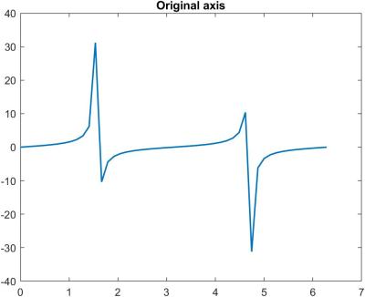


 and
and  , where
  , and
, and  .
.![U =[ u_1,\dots,u_m]](https://s0.wp.com/latex.php?latex=U+%3D%5B+u_1%2C%5Cdots%2Cu_m%5D&bg=ffffff&fg=222222&s=0&c=20201002) and
and ![V = [v_1,\dots, v_n]](https://s0.wp.com/latex.php?latex=V+%3D+%5Bv_1%2C%5Cdots%2C+v_n%5D&bg=ffffff&fg=222222&s=0&c=20201002) . The
. The  are called the singular values of
  and
and  are the left and right singular vectors. We have
  ,
,  . The matrix
  is unique but
 ![\notag \Sigma = \left[\begin{array}{ccc}\sigma_1&&\\ &\ddots&\\& &\sigma_n\\\hline &\rule{0cm}{15pt} \text{\Large 0} & \end{array}\right] \mathrm{for}~ m \ge n, \quad \Sigma = \begin{bmatrix} \begin{array}{ccc|c@{\mskip5mu}}\sigma_1&&\\ &\ddots& & \text{\Large 0} \\& &\sigma_m\end{array}\\ \end{bmatrix} \mathrm{for}~ m \le n](https://s0.wp.com/latex.php?latex=%5Cnotag++%5CSigma+%3D+++++++%5Cleft%5B%5Cbegin%7Barray%7D%7Bccc%7D%5Csigma_1%26%26%5C%5C+%26%5Cddots%26%5C%5C%26+%26%5Csigma_n%5C%5C%5Chline+++++++++%26%5Crule%7B0cm%7D%7B15pt%7D+%5Ctext%7B%5CLarge+0%7D+%26++++++%5Cend%7Barray%7D%5Cright%5D++++++%5Cmathrm%7Bfor%7D%7E+m+%5Cge+n%2C+%5Cquad++++%5CSigma+%3D+++++%5Cbegin%7Bbmatrix%7D+++++++++%5Cbegin%7Barray%7D%7Bccc%7Cc%40%7B%5Cmskip5mu%7D%7D%5Csigma_1%26%26%5C%5C+%26%5Cddots%26+++++++++++++++%26+%5Ctext%7B%5CLarge+0%7D+++++++++++%5C%5C%26+%26%5Csigma_m%5Cend%7Barray%7D%5C%5C++++++%5Cend%7Bbmatrix%7D+%5Cmathrm%7Bfor%7D%7E+m+%5Cle+n+&bg=ffffff&fg=222222&s=0&c=20201002)
![\notag A = \left[\begin{array}{rr} 0 & \frac{4}{3}\\[\smallskipamount] -1 & -\frac{5}{3}\\[\smallskipamount] -2 & -\frac{2}{3} \end{array}\right] = \underbrace{ \displaystyle\frac{1}{3} \left[\begin{array}{rrr} 1 & -2 & -2\\ -2 & 1 & -2\\ -2 & -2 & 1 \end{array}\right] }_U \mskip5mu \underbrace{ \left[\begin{array}{cc} 2\,\sqrt{2} & 0\\ 0 & \sqrt{2}\\ 0 & 0 \end{array}\right] }_{\Sigma} \mskip5mu \underbrace{ \displaystyle\frac{1}{\sqrt{2}} \left[\begin{array}{cc} 1 & 1\\ 1 & -1 \end{array}\right] }_{V^T}.](https://s0.wp.com/latex.php?latex=%5Cnotag+A+%3D+%5Cleft%5B%5Cbegin%7Barray%7D%7Brr%7D+0+%26+%5Cfrac%7B4%7D%7B3%7D%5C%5C%5B%5Csmallskipamount%5D++++++++++++++++++++++++-1+%26+-%5Cfrac%7B5%7D%7B3%7D%5C%5C%5B%5Csmallskipamount%5D++++++++++++++++++++++++-2+%26+-%5Cfrac%7B2%7D%7B3%7D+%5Cend%7Barray%7D%5Cright%5D+%3D+%5Cunderbrace%7B+%5Cdisplaystyle%5Cfrac%7B1%7D%7B3%7D+%5Cleft%5B%5Cbegin%7Barray%7D%7Brrr%7D+1+%26+-2+%26+-2%5C%5C+-2+%26+1+%26+-2%5C%5C+-2+%26+-2+%26+1+%5Cend%7Barray%7D%5Cright%5D+%7D_U+%5Cmskip5mu+%5Cunderbrace%7B+%5Cleft%5B%5Cbegin%7Barray%7D%7Bcc%7D+2%5C%2C%5Csqrt%7B2%7D+%26+0%5C%5C+0+%26+%5Csqrt%7B2%7D%5C%5C+0+%26+0+%5Cend%7Barray%7D%5Cright%5D+%7D_%7B%5CSigma%7D+%5Cmskip5mu+%5Cunderbrace%7B+%5Cdisplaystyle%5Cfrac%7B1%7D%7B%5Csqrt%7B2%7D%7D+%5Cleft%5B%5Cbegin%7Barray%7D%7Bcc%7D+1+%26+1%5C%5C+1+%26+-1++%5Cend%7Barray%7D%5Cright%5D+%7D_%7BV%5ET%7D.+&bg=ffffff&fg=222222&s=0&c=20201002)
 , where
  is the number of nonzero singular values. Since the
  for both norms, giving
 . The range space and null space of

 rank-
rank-

 terms gives the best rank-
 .
. implies
 (modulo
  zeros in the latter case), and the singular vectors are eigenvectors. Moreover, the eigenvalues of the
  matrix
 additional zeros if
  , and the eigenvectors of
  can be expressed in terms of the SVD as
 , where
  is solved by
  , and when
  this is an underdetermined system and
  , where
  is the polar decomposition and
  is unique. This connection between the SVD and the polar decomposition is useful both theoretically and computationally.
 we have the Taylor expansion
 is the imaginary unit. Assume that
  are real. Then equating real and imaginary parts in
  and
and  . This means that for small
 . So a single evaluation of
  , as well as a good approximation to
  if we need it.
 so it is less accurate than the complex step approximation for a given
  and
and 
 .
. with
with  , we plot in the figure below the relative error for the finite difference, in blue, and the relative error for the complex step approximation, in orange, for
  . The dotted lines show
  ). The finite difference error decreases with
  ; thereafter the error grows, giving the characteristic V-shaped error curve. The complex step error decreases steadily until it is of order
  , and for each
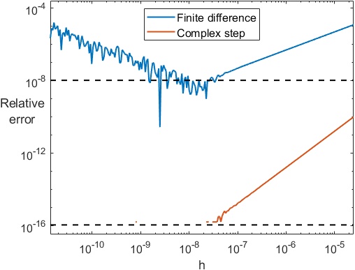
 ) without any ill effects from roundoff.
 are real then (Al-Mohy and Higham, 2010)
 is the Fréchet derivative of
  term can lead to damaging subtractive cancellation.
 is nonsingular then the identity
  shows that
 , where
  are
are  . We might expect that
  for some
 . The condition that
  be nonsingular is
  (as can also be seen from
  , derived in
 . Inverting this equation and applying the previous result gives
 . This is known as the Sherman–Morrison formula. It explicitly identifies the rank-
 and
and  (where
  is the
  , we have
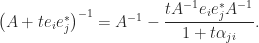
 and
and  are likely to give the maximum, which means that the inverse of an upper triangular matrix is likely to be most sensitive to perturbations in the
  element of the matrix. To illustrate, we consider the matrix
![\notag T = \left[\begin{array}{rrrr} 1 & -1 & -2 & -3\\ 0 & 1 & -4 & -5\\ 0 & 0 & 1 & -6\\ 0 & 0 & 0 & 1 \end{array}\right]](https://s0.wp.com/latex.php?latex=%5Cnotag++T+%3D++%5Cleft%5B%5Cbegin%7Barray%7D%7Brrrr%7D+++1+%26+-1+%26+-2+%26+-3%5C%5C+++0+%26+1+%26+-4+%26+-5%5C%5C+++0+%26+0+%26+1+%26+-6%5C%5C+++0+%26+0+%26+0+%26+1+++%5Cend%7Barray%7D%5Cright%5D+&bg=ffffff&fg=222222&s=0&c=20201002)
 element of the following matrix is
  :
:![\notag \left[\begin{array}{cccc} 0.044 & 0.029 & 0.006 & 0.001 \\ 0.063 & 0.041 & 0.009 & 0.001 \\ 0.322 & 0.212 & 0.044 & 0.007 \\ 2.258 & 1.510 & 0.321 & 0.053 \\ \end{array}\right]](https://s0.wp.com/latex.php?latex=%5Cnotag+++%5Cleft%5B%5Cbegin%7Barray%7D%7Bcccc%7D++0.044++%26++0.029++%26++0.006++%26++0.001++%5C%5C++0.063++%26++0.041++%26++0.009++%26++0.001++%5C%5C++0.322++%26++0.212++%26++0.044++%26++0.007++%5C%5C++2.258++%26++1.510++%26++0.321++%26++0.053++%5C%5C+++%5Cend%7Barray%7D%5Cright%5D+&bg=ffffff&fg=222222&s=0&c=20201002)
 entry is the most sensitive to perturbation.
 , where
  . This perturbation has rank at most
  is nonsingular then
  is nonsingular and
 , so if
  and
and  in
in  flops, as opposed to the
  flops required to factorize
  and
and  such that
  and
and  are both defined. The associative law for matrix multiplication gives
  , or
, or  , which can be written as
  . Postmultiplying by
 and
and  gives the special case of the Sherman–Morrison–Woodbury formula with
  .
.
 is
is  by looking at
  .
.
![\notag \begin{aligned} \begin{bmatrix} A & U \\ V^* & -W^{-1} \end{bmatrix}^{-1} &= \begin{bmatrix} I & -A^{-1}U \\ 0 & I \end{bmatrix}. \begin{bmatrix} A^{-1} & 0 \\ 0 & -(W^{-1} + V^*A^{-1}U)^{-1} \end{bmatrix} \begin{bmatrix} I & 0 \\ -V^*A^{-1} & I \end{bmatrix}\\[\smallskipamount] &= \begin{bmatrix} A^{-1} - A^{-1}U(W^{-1} + V^*A^{-1}U)^{-1}V^*A^{-1} & A^{-1}U(W^{-1} + V^*A^{-1U})^{-1} \\ (W^{-1} + V^*A^{-1}U)^{-1} V^*A^{-1} & -(W^{-1} + V^*A^{-1}U)^{-1} \end{bmatrix}. \end{aligned}](https://s0.wp.com/latex.php?latex=%5Cnotag+%5Cbegin%7Baligned%7D++++%5Cbegin%7Bbmatrix%7D+A+%26+U+%5C%5C+V%5E%2A+%26+-W%5E%7B-1%7D+%5Cend%7Bbmatrix%7D%5E%7B-1%7D+++++%26%3D++++%5Cbegin%7Bbmatrix%7D+I+%26+-A%5E%7B-1%7DU+%5C%5C+0+%26+I+%5Cend%7Bbmatrix%7D.++++%5Cbegin%7Bbmatrix%7D+A%5E%7B-1%7D+%26+0+%5C%5C+0+%26+-%28W%5E%7B-1%7D+%2B+V%5E%2AA%5E%7B-1%7DU%29%5E%7B-1%7D+%5Cend%7Bbmatrix%7D++++%5Cbegin%7Bbmatrix%7D+I+%26+0+%5C%5C+-V%5E%2AA%5E%7B-1%7D+%26+I+%5Cend%7Bbmatrix%7D%5C%5C%5B%5Csmallskipamount%5D+++++%26%3D++++%5Cbegin%7Bbmatrix%7D+A%5E%7B-1%7D+-+A%5E%7B-1%7DU%28W%5E%7B-1%7D+%2B+V%5E%2AA%5E%7B-1%7DU%29%5E%7B-1%7DV%5E%2AA%5E%7B-1%7D+%26++++++++++++++++++++A%5E%7B-1%7DU%28W%5E%7B-1%7D+%2B+V%5E%2AA%5E%7B-1U%7D%29%5E%7B-1%7D+%5C%5C++++++++++%28W%5E%7B-1%7D+%2B+V%5E%2AA%5E%7B-1%7DU%29%5E%7B-1%7D+V%5E%2AA%5E%7B-1%7D+%26+-%28W%5E%7B-1%7D+%2B+V%5E%2AA%5E%7B-1%7DU%29%5E%7B-1%7D++++++%5Cend%7Bbmatrix%7D.+%5Cend%7Baligned%7D+&bg=ffffff&fg=222222&s=0&c=20201002)
 block we see the right-hand side of a Sherman–Morrison–Woodbury-like formula, but it is not immediately clear how this relates to
 ![P = \bigl[\begin{smallmatrix} 0 & I \\ I & 0 \end{smallmatrix} \bigr]](https://s0.wp.com/latex.php?latex=P+%3D+%5Cbigl%5B%5Cbegin%7Bsmallmatrix%7D+0+%26+I+%5C%5C+I+%26+0+%5Cend%7Bsmallmatrix%7D+%5Cbigr%5D&bg=ffffff&fg=222222&s=0&c=20201002) , and note that
, and note that  . Then
 denoting a block whose value does not matter,
 . Equating our two formulas for
  gives
gives
 is nonsingular.
 , so the perturbation must be positive semidefinite. In
  , with
  is the Schur complement of
 is nonsingular. Note that the formula is not symmetric when
  and
and  . This variant can also be obtained by replacing
  in the Sherman–Morrison–Woodbury formula.
 , partitioning into
 ![\notag A = \left[\begin{array}{cc|cc} a_{11} & a_{12} & a_{13} & a_{14}\\ a_{21} & a_{22} & a_{23} & a_{24}\\\hline a_{31} & a_{32} & a_{33} & a_{34}\\ a_{41} & a_{42} & a_{43} & a_{44}\\ \end{array}\right] = \begin{bmatrix} A_{11} & A_{12} \\ A_{21} & A_{22} \end{bmatrix},](https://s0.wp.com/latex.php?latex=%5Cnotag+++A+%3D+%5Cleft%5B%5Cbegin%7Barray%7D%7Bcc%7Ccc%7D+++++++++a_%7B11%7D+%26+a_%7B12%7D+%26+a_%7B13%7D+%26+a_%7B14%7D%5C%5C+++++++++a_%7B21%7D+%26+a_%7B22%7D+%26+a_%7B23%7D+%26+a_%7B24%7D%5C%5C%5Chline+++++++++a_%7B31%7D+%26+a_%7B32%7D+%26+a_%7B33%7D+%26+a_%7B34%7D%5C%5C+++++++++a_%7B41%7D+%26+a_%7B42%7D+%26+a_%7B43%7D+%26+a_%7B44%7D%5C%5C+++++++++%5Cend%7Barray%7D%5Cright%5D++++%3D++%5Cbegin%7Bbmatrix%7D+++++++++A_%7B11%7D+%26+A_%7B12%7D+%5C%5C+++++++++A_%7B21%7D+%26+A_%7B22%7D++++++++%5Cend%7Bbmatrix%7D%2C+&bg=ffffff&fg=222222&s=0&c=20201002)
![\notag A = \left[\begin{array}{c|ccc} a_{11} & a_{12} & a_{13} & a_{14}\\\hline a_{21} & a_{22} & a_{23} & a_{24}\\ a_{31} & a_{32} & a_{33} & a_{34}\\ a_{41} & a_{42} & a_{43} & a_{44}\\ \end{array}\right] = \begin{bmatrix} A_{11} & A_{12} \\ A_{21} & A_{22} \end{bmatrix},](https://s0.wp.com/latex.php?latex=%5Cnotag+++A+%3D+%5Cleft%5B%5Cbegin%7Barray%7D%7Bc%7Cccc%7D+++++++++a_%7B11%7D+%26+a_%7B12%7D+%26+a_%7B13%7D+%26+a_%7B14%7D%5C%5C%5Chline+++++++++a_%7B21%7D+%26+a_%7B22%7D+%26+a_%7B23%7D+%26+a_%7B24%7D%5C%5C+++++++++a_%7B31%7D+%26+a_%7B32%7D+%26+a_%7B33%7D+%26+a_%7B34%7D%5C%5C+++++++++a_%7B41%7D+%26+a_%7B42%7D+%26+a_%7B43%7D+%26+a_%7B44%7D%5C%5C+++++++++%5Cend%7Barray%7D%5Cright%5D++++%3D++%5Cbegin%7Bbmatrix%7D+++++++++A_%7B11%7D+%26+A_%7B12%7D+%5C%5C+++++++++A_%7B21%7D+%26+A_%7B22%7D++++++++%5Cend%7Bbmatrix%7D%2C+&bg=ffffff&fg=222222&s=0&c=20201002)
 is a scalar,
  is a column vector, and
  is a row vector.
 of two block matrices
  and
and  of the same dimension is obtained by adding blockwise as long as
  and
and  have the same dimensions for all
  ,
, of an
of an  matrix
  matrix
  as long as the products
  are all defined. In this case the matrices
 we can write
 have the correct form for a unit lower triangular matrix and likewise the first row and column of
  of the
  Schur complement
  then
then  is an LU factorization of
 is upper triangular then so are
  and
and  . By taking
  this formula can be used to construct a divide and conquer algorithm for computing
  .
. , a fact that will be used in the next section.
 and
and  are defined. Taking determinants gives the formula
  . In particular we can take
  ,
,  , for
, for  , giving
  .
. ) then
 involutory matrix. And if

![\notag \mathrm{e}^X = \left[\begin{array}{cc} \cosh\sqrt{AB} & A (\sqrt{BA})^{-1} \sinh \sqrt{BA} \\[\smallskipamount] B(\sqrt{AB})^{-1} \sinh \sqrt{AB} & \cosh\sqrt{BA} \end{array}\right],](https://s0.wp.com/latex.php?latex=%5Cnotag+++%5Cmathrm%7Be%7D%5EX+%3D+%5Cleft%5B%5Cbegin%7Barray%7D%7Bcc%7D+++++++++++++++++++%5Ccosh%5Csqrt%7BAB%7D+%26+A+%28%5Csqrt%7BBA%7D%29%5E%7B-1%7D+%5Csinh+%5Csqrt%7BBA%7D++++++++++++++++++++++++%5C%5C%5B%5Csmallskipamount%5D+++++++++++++++++++++++B%28%5Csqrt%7BAB%7D%29%5E%7B-1%7D+%5Csinh+%5Csqrt%7BAB%7D+%26++++++++++++++++++++++%5Ccosh%5Csqrt%7BBA%7D++++++++++++++++++%5Cend%7Barray%7D%5Cright%5D%2C+&bg=ffffff&fg=222222&s=0&c=20201002)
 denotes any square root of
  . With
  , this formula arises in the solution of the ordinary differential equation initial value problem
  ,
,  ,
,  ,
, . The eigenvalues of

 ),
), ),
), that is,
  .
. for every such
  and determinant
![v = e = [1,1,\dots,1]^T](https://s0.wp.com/latex.php?latex=v+%3D+e+%3D+%5B1%2C1%2C%5Cdots%2C1%5D%5ET&bg=ffffff&fg=222222&s=0&c=20201002) , for which
, for which  . For
. For  we obtain the matrices
![\notag \begin{gathered} \left[\begin{array}{@{\mskip2mu}rr@{\mskip2mu}} 0 & -1 \\ -1 & 0 \end{array}\right], \quad \displaystyle\frac{1}{3} \left[\begin{array}{@{\mskip2mu}rrr@{\mskip2mu}} 1 & -2 & -2\\ -2 & 1 & -2\\ -2 & -2 & 1\\ \end{array}\right], \quad \displaystyle\frac{1}{2} \left[\begin{array}{@{\mskip2mu}rrrr@{\mskip2mu}} 1 & -1 & -1 & -1\\ -1 & 1 & -1 & -1\\ -1 & -1 & 1 & -1\\ -1 & -1 & -1 & 1\\ \end{array}\right], \\ \displaystyle\frac{1}{5} \left[\begin{array}{@{\mskip2mu}rrrrr@{\mskip2mu}} 3 & -2 & -2 & -2 & -2\\ -2 & 3 & -2 & -2 & -2\\ -2 & -2 & 3 & -2 & -2\\ -2 & -2 & -2 & 3 & -2\\ -2 & -2 & -2 & -2 & 3 \end{array}\right], \quad \displaystyle\frac{1}{3} \left[\begin{array}{@{\mskip2mu}rrrrrr@{\mskip2mu}} 2 & -1 & -1 & -1 & -1 & -1\\ -1 & 2 & -1 & -1 & -1 & -1\\ -1 & -1 & 2 & -1 & -1 & -1\\ -1 & -1 & -1 & 2 & -1 & -1\\ -1 & -1 & -1 & -1 & 2 & -1\\ -1 & -1 & -1 & -1 & -1 & 2 \end{array}\right]. \end{gathered}](https://s0.wp.com/latex.php?latex=%5Cnotag++++%5Cbegin%7Bgathered%7D++++++++%5Cleft%5B%5Cbegin%7Barray%7D%7B%40%7B%5Cmskip2mu%7Drr%40%7B%5Cmskip2mu%7D%7D++++++++++++++++++++++0+%26+-1+%5C%5C+-1+%26+0++++++++%5Cend%7Barray%7D%5Cright%5D%2C+%5Cquad+++%5Cdisplaystyle%5Cfrac%7B1%7D%7B3%7D++++++++%5Cleft%5B%5Cbegin%7Barray%7D%7B%40%7B%5Cmskip2mu%7Drrr%40%7B%5Cmskip2mu%7D%7D+++++++++++++++++++++++1+%26++-2+%26++-2%5C%5C++++++++++++++++++++++-2+%26+++1+%26++-2%5C%5C++++++++++++++++++++++-2+%26++-2+%26+++1%5C%5C++++++++%5Cend%7Barray%7D%5Cright%5D%2C+%5Cquad++++%5Cdisplaystyle%5Cfrac%7B1%7D%7B2%7D++++++++%5Cleft%5B%5Cbegin%7Barray%7D%7B%40%7B%5Cmskip2mu%7Drrrr%40%7B%5Cmskip2mu%7D%7D++++++++++++++++++++++++1+%26+++-1+%26+++-1+%26+++-1%5C%5C+++++++++++++++++++++++-1+%26++++1+%26+++-1+%26+++-1%5C%5C+++++++++++++++++++++++-1+%26+++-1+%26++++1+%26+++-1%5C%5C+++++++++++++++++++++++-1+%26+++-1+%26+++-1+%26++++1%5C%5C++++++++%5Cend%7Barray%7D%5Cright%5D%2C+%5C%5C+++%5Cdisplaystyle%5Cfrac%7B1%7D%7B5%7D++++++++%5Cleft%5B%5Cbegin%7Barray%7D%7B%40%7B%5Cmskip2mu%7Drrrrr%40%7B%5Cmskip2mu%7D%7D++++3+%26+-2+%26+-2+%26+-2+%26+-2%5C%5C+-2+%26+3+%26+-2+%26+-2+%26++++-2%5C%5C+-2+%26+-2+%26+3+%26+-2+%26+-2%5C%5C+-2+%26+-2+%26+-2+%26+3+%26+-2%5C%5C+-2+%26+-2+%26+-2+%26+-2+%26+3+++%5Cend%7Barray%7D%5Cright%5D%2C+%5Cquad++%5Cdisplaystyle%5Cfrac%7B1%7D%7B3%7D+%5Cleft%5B%5Cbegin%7Barray%7D%7B%40%7B%5Cmskip2mu%7Drrrrrr%40%7B%5Cmskip2mu%7D%7D+++2+%26+-1+%26+-1+%26+-1+%26+-1+%26+-1%5C%5C+-1+%26+2+%26+-1+%26+-1+%26+-1+%26+-1%5C%5C+++-1+%26+-1+%26+2+%26+-1+%26+-1+%26+-1%5C%5C+-1+%26+-1+%26+-1+%26+2+%26+-1+%26+-1%5C%5C+-1+%26+-1+%26+-1+%26+-1+%26+2+%26+-1%5C%5C+++-1+%26+-1+%26+-1+%26+-1+%26+-1+%26+2+%5Cend%7Barray%7D%5Cright%5D.++++%5Cend%7Bgathered%7D+&bg=ffffff&fg=222222&s=0&c=20201002)
 times a Hadamard matrix.
 , as illustrated in the following diagram, which explains why
  , where
  is orthogonal to
  , so the component of
  , the
, the  , which has
  position. In this case premultiplying a vector by
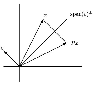
 . Since
  , and we exclude the trivial case
  . Now
. Now
 for some
  . Now with
  we have
 ,
,

 ?
? and one will be
  . This means that
  , where
  . It is natural to look for a square root of the form
  . Setting
  , and hence
  . As expected, these two square roots are complex even though
  gives the following square root of the matrix above corresponding to
  with
with ![\notag X = \displaystyle\frac{1}{3} \left[\begin{array}{@{\mskip2mu}rrr} 2+\mathrm{i} & -1+\mathrm{i} & -1+\mathrm{i}\\ -1+\mathrm{i} & 2+\mathrm{i} & -1+\mathrm{i}\\ -1+\mathrm{i} & -1+\mathrm{i} & 2+\mathrm{i} \end{array}\right].](https://s0.wp.com/latex.php?latex=%5Cnotag+X+%3D+%5Cdisplaystyle%5Cfrac%7B1%7D%7B3%7D+%5Cleft%5B%5Cbegin%7Barray%7D%7B%40%7B%5Cmskip2mu%7Drrr%7D+2%2B%5Cmathrm%7Bi%7D+%26+-1%2B%5Cmathrm%7Bi%7D+%26+-1%2B%5Cmathrm%7Bi%7D%5C%5C+-1%2B%5Cmathrm%7Bi%7D+%26+2%2B%5Cmathrm%7Bi%7D+%26+-1%2B%5Cmathrm%7Bi%7D%5C%5C+-1%2B%5Cmathrm%7Bi%7D+%26+-1%2B%5Cmathrm%7Bi%7D+%26+2%2B%5Cmathrm%7Bi%7D+%5Cend%7Barray%7D%5Cright%5D.+&bg=ffffff&fg=222222&s=0&c=20201002)
 and
and  . Then from the construction above we know that
  . Hence
 and so
  gives
gives  . Because
  , where
  , where
  , as
, as
 ” denotes the Moore–Penrose pseudoinverse. For
  (this is most easily proved using the SVD), and so
 is the orthogonal projector onto the range of
  (that is,
  ,
,  , and
, and  ). Hence, like a standard Householder matrix,
 ![Z = \bigl[\begin{smallmatrix} 1 & 2 & 3 & 4\\ 5 & 6 & 7 & 8 \end{smallmatrix}\bigr]^T](https://s0.wp.com/latex.php?latex=Z+%3D+%5Cbigl%5B%5Cbegin%7Bsmallmatrix%7D+1+%26+2+%26+3+%26+4%5C%5C+5+%26+6+%26+7+%26+8+%5Cend%7Bsmallmatrix%7D%5Cbigr%5D%5ET&bg=ffffff&fg=222222&s=0&c=20201002) :
:![\notag \displaystyle\frac{1}{5} \left[\begin{array}{@{\mskip2mu}rrrr@{\mskip2mu}} -2 & -4 & -1 & 2\\ -4 & 2 & -2 & -1\\ -1 & -2 & 2 & -4\\ 2 & -1 & -4 & -2 \end{array}\right].](https://s0.wp.com/latex.php?latex=%5Cnotag+%5Cdisplaystyle%5Cfrac%7B1%7D%7B5%7D+%5Cleft%5B%5Cbegin%7Barray%7D%7B%40%7B%5Cmskip2mu%7Drrrr%40%7B%5Cmskip2mu%7D%7D+-2+%26+-4+%26+-1+%26+2%5C%5C+-4+%26+2+%26+-2+%26+-1%5C%5C+-1+%26+-2+%26+2+%26+-4%5C%5C+2+%26+-1+%26+-4+%26+-2+%5Cend%7Barray%7D%5Cright%5D.+&bg=ffffff&fg=222222&s=0&c=20201002)
 times, where
  . Hence
  and
and  .
. ,
,
 is symmetric positive definite. This formula neatly generalizes the formula for a standard Householder matrix for
  (
( ) one can construct a block Householder matrix
 ,
,  ,
,  , and
, and
![[u^T~v^T]^T](https://s0.wp.com/latex.php?latex=%5Bu%5ET%7Ev%5ET%5D%5ET&bg=ffffff&fg=222222&s=0&c=20201002) .
. ) then a unitary matrix of the form
  (in their notation) can be constructed so that
  . They use this result to prove the existence of the Schur decomposition. The first systematic use of Householder matrices for computational purposes was by Householder (1958) who used them to construct the QR factorization.
