What’s New in MATLAB R2020a and R2020b?

In this post I discuss new features in MATLAB R2020a and R2020b. As usual in this series, I focus on a few of the features most relevant to my work. See the release notes for a detailed list of the many changes in MATLAB and its toolboxes.

Exportgraphics (R2020a)

The exportgraphics function is very useful for saving to a file a tightly cropped version of a figure with the border white instead of gray. Simple usages are

exportgraphics(gca,'image.pdf')
exportgraphics(gca,'image.jpg','Resolution',200)

I have previously used the export_fig function, which is not built into MATLAB but is available from File Exchange; I think I will be using exportgraphics instead from now on.

Svdsketch (R2020b)

The new svdsketch function computes the singular value decomposition (SVD) $USV^T$ of a low rank approximation to a matrix ( $U$ and $V$ orthogonal, $S$ diagonal with nonnegative diagonal entries). It is mainly intended for use with matrices that are close to having low rank, as is the case in various applications.

This function uses a randomized algorithm that computes a sketch of the given $m$ -by- $n$ matrix $A$ , which is essentially a product $Q^TA$ , where $Q$ is an orthonormal basis for the product $A\Omega$ , where $\Omega$ is a random $n$ -by- $k$ matrix. The value of $k$ is chosen automatically to achieve $\|USV^T-A\|_F \le \mathrm{tol}\|A\|_F$ , where $\mathrm{tol}$ is a tolerance that defaults to $\epsilon^{1/4}$ and must not be less than $\epsilon^{1/2}$ , where $\epsilon$ is the machine epsilon ( $2\times 10^{-16}$ for double precision). The algorithm includes a power method iteration that refines the sketch before computing the SVD.

The output of the function is an SVD in which $U$ and $V$ are numerically orthogonal and the singular values in $S$ of size $\mathrm{tol}$ or larger are good approximations to singular values of $A$ , but smaller singular values in $S$ may not be good approximations to singular values of $A$ .

Here is an example. The code

n = 8; rng(1); 8; A = gallery('randsvd',n,1e8,3);
[U,S,V] = svdsketch(A,1e-3);
rel_res = norm(A-U*S*V')/norm(A)
singular_values = [svd(A) [diag(S); zeros(n-length(S),1)]]

produces the following output, with the exact singular values in the first column and the approximate ones in the second column:

rel_res =
   1.9308e-06
singular_values =
   1.0000e+00   1.0000e+00
   7.1969e-02   7.1969e-02
   5.1795e-03   5.1795e-03
   3.7276e-04   3.7276e-04
   2.6827e-05   2.6827e-05
   1.9307e-06            0
   1.3895e-07            0
   1.0000e-08            0

The approximate singular values are correct down to around $10^{-5}$ , which is more than the $10^{-3}$ requested. This is a difficult matrix for svdsketch because there is no clear gap in the singular values of $A$ .

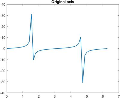
Axis Padding (R2020b)

The padding property of an axis puts some padding between the axis limits and the surrounding box. The code

x = linspace(0,2*pi,50); plot(x,tan(x),'linewidth',1.4)
title('Original axis')
axis padded, title('Padded axis')

produces the output

Turbo Colormap (2020b)

The default colormap changed from jet (the rainbow color map) to parula in R2014b (with a tweak in R2017a), because parula is more perceptually uniform and maintains information when printed in monochrome. The new turbo colormap is a more perceptually uniform version of jet, as these examples show. Notice that turbo has a longer transition through the greens and yellows. If you can’t give up on jet, use turbo instead.

Turbo:

Jet:

Parula:

ND Arrays (R2020b)

The new pagemtimes function performs matrix multiplication on pages of $n$ -dimensional arrays, while pagetranspose and pagectranspose carry out the transpose and conjugate transpose, respectively, on pages of $n$ -dimensional arrays.

Performance

Both releases report significantly improved speed of certain functions, including some of the ODE solvers.

One thought on “What’s New in MATLAB R2020a and R2020b?”

Thanks, Nick, for this and other posts. I use MATLAB a lot and was not aware of some of these enhancements. .