When Does Thresholding Preserve Positive Definiteness?

Does a symmetric positive definite matrix remain positive definite when we set one or more elements to zero? This question arises in thresholding, in which elements of absolute value less than some tolerance are set to zero. Thresholding is used in some applications to remove correlations thought to be spurious, so that only statistically significant ones are retained.

We will focus on the case where just one element is changed and consider an arbitrary target value rather than zero. Given an $n\times n$ symmetric positive definite matrix $A$ we define $A(t)$ to be the matrix resulting from adding $t$ to the $(i,j)$ and $(j,i)$ elements and we ask when is $A(t)$ positive definite. We can write

$\notag A(t) = A + t(e_i^{}e_j^T + e_j^{}e_i^T) \equiv A + tE_{ij},$

where $e_i$ is the $i$ th column of the identity matrix. The perturbation $E_{ij}$ has rank $2$ , with eigenvalues $-1$ , $1$ , and $0$ repeated $n-2$ times. Hence we can write $E_{ij}$ in the form $E_{ij} = pp^T - qq^T$ , where $p^Tp = q^Tq = 1$ and $p^Tq = 0$ . Adding $pp^T$ to $A$ causes each eigenvalue to increase or stay the same, while subtracting $qq^T$ decreases or leaves unchanged each eigenvalue. However, more is true: after each of these rank- $1$ perturbations the eigenvalues of the original and perturbed matrices interlace, by Weyl’s theorem. Hence, with the eigenvalues of $A$ ordered as $\lambda_n(A) \le \cdots \le \lambda_1(A)$ , we have (Horn and Johnson, Cor. 4.3.7)

$\notag \begin{aligned} \lambda_n(A(t)) &\le \lambda_{n-1}(A), \\ \lambda_{i+1}(A) &\le \lambda_i(A(t)) \le \lambda_{i-1}(A), \quad i = 2\colon n-1, \\ \lambda_2(A) &\le \lambda_1(A(t)). \end{aligned}$

Because $A$ is positive definite these inequalities imply that 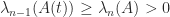$\lambda_{n-1}(A(t)) \ge \lambda_n(A) > 0$ , so $A(t)$ has at most one negative eigenvalue. Since $\det(A(t))$ is the product of the eigenvalues of $A(t)$ this means that $A(t)$ is positive definite precisely when $\det(A(t)) > 0$ .

There is a simple expression for $\det(A(t))$ , which follows from a lemma of Chan (1984), as explained by Georgescu, Higham, and Peters (2018):

$\notag \det(A(t)) = \det(A)\big(1+ 2t b_{ij} + t^2(b_{ij}^2-b_{ii}b_{jj})\big),$

where $B = A^{-1}$ . Hence the condition for $A(t)$ to be positive definite is

$\notag q_{ij}(t) = 1 + 2t b_{ij} + t^2(b_{ij}^2-b_{ii}b_{jj}) > 0.$

We can factorize

$\notag q_{ij}(t) = \Bigl( t\bigl(b_{ij} - \sqrt{b_{ii}b_{jj}}\bigr) + 1 \Bigr) \Bigl( t\bigl(b_{ij} + \sqrt{b_{ii}b_{jj}}\bigr) + 1 \Bigr),$

so $q_{ij}(t) > 0$ for

$\notag t\in \left( \displaystyle\frac{-1}{ \sqrt{b_{ii}b_{jj}} + b_{ij} }, \displaystyle\frac{1}{ \sqrt{b_{ii}b_{jj}} - b_{ij} } \right) =: I_{ij},$

where the endpoints are finite because $B$ , like $A$ , is positive definite and so $|b_{ij}| < \sqrt{b_{ii}b_{jj}}$ .

The condition for $A$ to remain positive definite when $a_{ij}$ is set to zero is $q_{ij}(-a_{ij}) > 0$ , or equivalently $-a_{ij} \in I_{ij}$ . To check either of these conditions we need just $b_{ij}$ , $b_{ii}$ , and $b_{jj}$ . These elements can be computed without computing the whole inverse by solving the equations $Ab_k = e_k$ for $k = i,j$ , for the $k$ th column $b_k$ of $B$ , making use of a Cholesky factorization of $A$ .

As an example, we consider the $4\times 4$ Lehmer matrix, which has $(i,j)$ element $i/j$ for $i \ge j$ :

$\notag A = \begin{bmatrix} 1 & \frac{1}{2} & \frac{1}{3} & \frac{1}{4} \\[3pt] \frac{1}{2} & 1 & \frac{2}{3} & \frac{1}{2} \\[3pt] \frac{1}{3} & \frac{2}{3} & 1 & \frac{3}{4} \\[3pt] \frac{1}{4} & \frac{1}{2} & \frac{3}{4} & 1 \end{bmatrix}.$

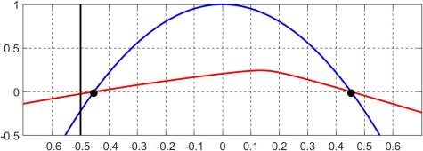
The smallest eigenvalue of $A$ is $0.208$ . Any off-diagonal element except the $(2,4)$ element can be zeroed without destroying positive definiteness, and if the $(2,4)$ element is zeroed then the new matrix has smallest eigenvalue $-0.0249$ . For $i=2$ and $j=4$ , the following plot shows in red $\lambda_{\min}(A(t))$ and in blue $q_{24}(t)$ ; the black dots are the endpoints of the closure of the interval $I_{24} = (-0.453,0.453)$ and the vertical black line is the value $-a_{24}$ . Clearly, $-a_{24}$ lies outside $I_{24}$ , which is why zeroing this element causes a loss of positive definiteness. Note that $I_{24}$ also tells us that we can increase $a_{24}$ to any number less than $0.953$ without losing definiteness.

Given a positive definite matrix and a set $S$ of elements to be modified we may wish to determine subsets (including a maximal subset) of $S$ for which the modifications preserve definiteness. Efficiently determining these subsets appears to be an open problem.

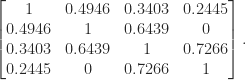
In practical applications thresholding may lead to an indefinite matrix. Definiteness must then be restored to obtain a valid correlation matrix. One way to do this is to find the nearest correlation matrix in the Frobenius norm such that the zeroed elements remain zero. This can be done by the alternating projections method with a projection to keep the zeroed elements fixed. Since the nearest correlation matrix is positive semidefinite, it is also desirable to to incorporate a lower bound $\delta > 0$ on the smallest eigenvalue, which corresponds to another projection. Both these projections are supported in the algorithm of Higham and Strabić (2016), implemented in the code at https://github.com/higham/anderson-accel-ncm. For the Lehmer matrix, the nearest correlation matrix with zero $(2,4)$ element and eigenvalues at least $\delta = 0.01$ is (to four significant figures)

$\notag \begin{bmatrix} 1 & 0.4946 & 0.3403 & 0.2445 \\ 0.4946 & 1 & 0.6439 & 0 \\ 0.3403 & 0.6439 & 1 & 0.7266 \\ 0.2445 & 0 & 0.7266 & 1 \end{bmatrix}.$

A related question is for what patterns of elements that are set to zero is positive definiteness guaranteed to be preserved for all positive definite $A$ ? Clearly, setting all the off-diagonal elements to zero preserves definiteness, since the diagonal of a positive definite matrix is positive. Guillot and Rajaratnam (2012) show that the answer to the question is that the new matrix must be a symmetric permutation of a block diagonal matrix. However, for particular $A$ this restriction does not necessarily hold, as the Lehmer matrix example shows.

References

Tony F. Chan, On the Existence and Computation of $LU$ -Factorizations with Small Pivots, Math. Comp. 42(166), 535–547, 1984.
Dan I. Georgescu, Nicholas J. Higham, and Gareth W. Peters, Explicit Solutions to Correlation Matrix Completion Problems, with an Application to Risk Management and Insurance, Roy. Soc. Open Sci. 5(3), 1–11, 2018
Dominique Guillot and Bala Rajaratnam, Retaining Positive Definiteness in Thresholded Matrices, Linear Algebra Appl. 436(11), 4143–4160, 2012.
Nicholas J. Higham and Nataša Strabić, Anderson Acceleration of the Alternating Projections Method for Computing the Nearest Correlation Matrix, Numer. Algorithms 72(4), 1021–1042, 2016. Sections 3.1, 3.2.
Roger A. Horn and Charles R. Johnson, Matrix Analysis, second edition, Cambridge University Press, 2013. My review of the second edition.

References

Share this:

Related

Leave a comment Cancel reply