What Is the Logarithmic Norm?

The logarithmic norm of a matrix $A\in\mathbb{C}^{n\times n}$ (also called the logarithmic derivative) is defined by

$\notag \mu(A) = \displaystyle\lim_{\epsilon \to 0+} \frac{ \|I + \epsilon A\| - 1}{\epsilon},$

where the norm is assumed to satisfy $\|I\| = 1$ .

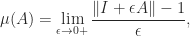
Note that the limit is taken from above. If we take the limit from below then we obtain a generally different quantity: writing $\delta = -\epsilon$ ,

$\notag \displaystyle\lim_{\epsilon \to 0-} \frac{ \|I + \epsilon A\| - 1}{\epsilon} = \lim_{\delta \to 0+} \frac{ \|I - \delta A\| - 1}{-\delta} = -\mu(-A).$

The logarithmic norm is not a matrix norm; indeed it can be negative: $\mu(-I) = -1$ .

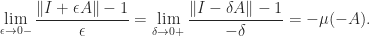
The logarithmic norm can also be expressed in terms of the matrix exponential.

Lemma 1. For $A\in\mathbb{C}^{n\times n}$ ,

$\notag \mu(A) = \displaystyle\lim_{\epsilon\to 0+} \frac{\log\, \| \mathrm{e}^{\epsilon A}\|} {\epsilon} = \lim_{\epsilon\to 0+} \frac{\| \mathrm{e}^{\epsilon A}\| - 1} {\epsilon}.$

Properties

We give some basic properties of the logarithmic norm.

It is easy to see that

$\notag -\|A\| \le \mu(A) \le \|A\|. \qquad (1)$

For $z\in\mathbb{C}$ , we define $\mathrm{sign}(z) = z/|z|$ for $z\ne 0$ and $\mathrm{sign}(0) = 0$ .

Lemma 2. For $A,B\in\mathbb{C}^{n\times n}$ and $\lambda\in\mathbb{C}$ ,

$\mu(\lambda A) = |\lambda| \mu\bigl(\mathrm{sign}(\lambda)A\bigr)$ ,

$\mu(A + \lambda I) = \mu(A) + \mathrm{Re}\,\lambda$ ,

$\mu(A + B ) \le \mu(A) + \mu(B)$ ,

$|\mu(A) - \mu(B)| \le \|A - B\|$ .

The next result shows the crucial property that $\mu(A)$ features in an easily evaluated bound for the norm of $\mathrm{e}^{At}$ and that, moreover, $\mu(A)$ is the smallest constant that can appear in this bound.

Theorem 3. For $A\in\mathbb{C}^{n\times n}$ and a consistent matrix norm,

$\notag \|\mathrm{e}^{At}\| \le \mathrm{e}^{\mu(A)t}, \quad t\ge0. \qquad (2)$

Moreover,

$\notag \mu(A) = \min\{\, \theta\in\mathbb{R}: \|\mathrm{e}^{At}\| \le \mathrm{e}^{\theta t} ~\mathrm{for~all}~t\ge 0 \,\}.$

Proof. Given any $\delta > 0$ , by Lemma 1 there exists $h > 0$ such that

$\notag \displaystyle\frac{ \| \mathrm{e}^{At}\| - 1}{t} - \mu(A) < \delta, \quad t\in[0,h],$

or

$\notag \| \mathrm{e}^{At}\| \le 1 + (\mu(A) + \delta)t \le \mathrm{e}^{(\mu(A) + \delta)t}, \quad t\in[0,h]$

(since $\mathrm{e}^x \ge 1+x$ for all $x$ ). Then for any integer $k$ , $\|\mathrm{e}^{Atk}\| = \|( \mathrm{e}^{At})^k\| \le \| \mathrm{e}^{At}\|^k \le \mathrm{e}^{(\mu(A) + \delta)tk}$ , and hence $\|\mathrm{e}^{At}\| \le \mathrm{e}^{(\mu(A) + \delta)t}$ holds for all $t\in[0,\infty)$ . Since $\delta$ is arbitrary, it follows that $\|\mathrm{e}^{At}\| \le \mathrm{e}^{\mu(A)t}$ .

Finally, if $\| \mathrm{e}^{At}\| \le \mathrm{e}^{\theta t}$ for all $t\ge 0$ then $(\| \mathrm{e}^{At}\| -1)/t\le (\mathrm{e}^{\theta t}-1)/t$ for all $t\ge0$ and taking $\lim_{t\to 0+}$ we conclude that $\mu(A) \le (d/dt) \mathrm{e}^{\theta t}\mid_{t = 0} \,= \theta$ .

The logarithmic norm was introduced by Dahlquist (1958) and Lozinskii (1958) in order to obtain error bounds for numerical methods for solving differential equations. The bound (2) can alternatively be proved by using differential inequalities (see Söderlind (2006)). Not only is (2) sharper than $\|\mathrm{e}^{At}\| \le \mathrm{e}^{\|A\|t}$ , but $\mathrm{e}^{\|A\|t}$ is increasing in $t$ while $\mathrm{e}^{\mu(A)t}$ potentially decays, since $\mu(A) < 0$ is possible.

The spectral abscissa is defined by

$\notag \alpha(A) = \max \{\, \mathrm{Re} \lambda : \lambda \in \Lambda(A)\,\},$

where $\Lambda(A)$ denotes the spectrum of $A$ (the set of eigenvalues). Whereas the norm bounds the spectral radius ( $\rho(A) \le \|A\|$ ), the logarithmic norm bounds the spectral abscissa, as shown by the next result.

Theorem 4. For $A\in\mathbb{C}^{n\times n}$ and a consistent matrix norm,

$\notag -\mu(-A) \le \alpha(A) \le \mu(A).$

Combining (1) with (2) gives

$\notag -\|A\| \le -\mu(-A) \le \alpha(A) \le \mu(A) \le \|A\|.$

In view of Lemma 1, the logarithmic norm $\mu(A)$ can be expressed as the one-sided derivative of $\|\mathrm{e}^{tA}\|$ at $t = 0$ , so $\mu(A)$ determines the initial rate of change of $\|\mathrm{e}^{tA}\|$ (as well as providing the bound $\mathrm{e}^{\mu(A)t}$ for all $t$ ). The long-term behavior is determined by the spectral abscissa $\alpha(A)$ , since $\|\mathrm{e}^{tA}\| \to 0$ as $t\to\infty$ if and only if $\alpha(A) < 0$ , which can be proved using the Jordan canonical form.

The next result provides a bound on the norm of the inverse of a matrix in terms of the logarithmic norm.

Theorem 5. For a nonsingular matrix $A\in\mathbb{C}^{n\times n}$ and a subordinate matrix norm, if $\mu(A) < 0$ or $\mu(-A) < 0$ then

$\notag \|A^{-1}\| \le \displaystyle\frac{1}{\max\bigl(-\mu(A),-\mu(-A)\bigr)}. \qquad (3)$

Formulas for Logarithmic Norms

Explicit formulas are available for the logarithmic norm s corresponding to the $1$ , $2$ , and $\infty$ -norms.

Theorem 6. For $A\in\mathbb{C}^{n\times n}$ ,

$\notag \begin{aligned} \mu_1(A) &= \max_j \biggl( \sum_{i\ne j} |a_{ij}| + \mathrm{Re}\, a_{jj} \biggr ),\\ \mu_{\infty}(A) &= \max_i \biggl( \sum_{j\ne i} |a_{ij}| + \mathrm{Re}\, a_{ii} \biggr ),\\ \mu_2(A) &= \lambda_{\max}\Bigl( \frac{A+A^*}{2} \Bigr), \qquad (4) \end{aligned}$

where $\lambda_{\max}$ denotes the largest eigenvalue of a Hermitian matrix.

Proof. We have

$\notag \begin{aligned} \mu_{\infty}(A) &= \lim_{\epsilon \to 0+} \frac{ \|I + \epsilon A\|_{\infty} - 1}{\epsilon}\\ &= \lim_{\epsilon \to 0+} \frac{ \max_i \bigl(\sum_{j\ne i} |\epsilon a_{ij}| + |1 + \epsilon a_{ii}| \bigr) -1}{\epsilon}\\ &= \lim_{\epsilon \to 0+} \frac{ \max_i \bigl(\sum_{j\ne i} |\epsilon a_{ij}| + \sqrt{(1 + \epsilon\mathrm{Re}\, a_{ii})^2 + (\epsilon\mathrm{Im}\,a_{ii})^2}\, \bigr) -1}{\epsilon}\\ &= \lim_{\epsilon \to 0+} \frac{ \max_i \bigl( \sum_{j\ne i} |\epsilon a_{ij}| + \epsilon\mathrm{Re}\, a_{ii} + O(\epsilon^2) \bigr)}{\epsilon}\\ &= \max_i \biggl( \sum_{j\ne i} |a_{ij}| + \mathrm{Re}\, a_{ii} \biggr ). \end{aligned}$

The formula for $\mu_1(A)$ follows, since $\|A\|_1 = \|A^*\|_\infty$ implies $\mu_1(A) = \mu_{\infty}(A^*)$ . For the $2$ -norm, using $\|A\|_2 = \rho(A^*A)^{1/2}$ , we have

$\notag \begin{aligned} \mu_2(A) &= \lim_{\epsilon \to 0+} \frac{ \|I + \epsilon A\|_2 - 1}{\epsilon}\\ &= \lim_{\epsilon \to 0+} \frac{ \rho\bigl( I + \epsilon(A+A^*) + \epsilon^2 A^*A\bigr)^{1/2} -1} {\epsilon}\\ &= \lim_{\epsilon \to 0+} \frac{ 1 + \frac{1}{2}\epsilon\lambda_{\max}(A+A^*) + O(\epsilon^2) -1} {\epsilon}\\ &= \lambda_{\max}\Bigl( \frac{A+A^*}{2} \Bigr). \end{aligned}$

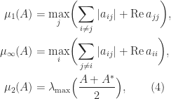
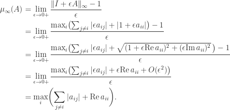
As a special case of (4), if $A$ is normal, so that $A = QDQ^*$ with $Q$ unitary and $D = \mathrm{diag}(\lambda_i)$ , then $\mu_2(A) = \max_i (\lambda_i + \overline{\lambda_i})/2 = \max_i \mathrm{Re} \lambda_i = \alpha(A)$ .

We can make some observations about $\mu_\infty(A)$ for $A\in\mathbb{R}^{n\times n}$ .

If $A\ge 0$ then $\mu_\infty(A) = \|A\|_\infty$ .
$\mu_\infty(A) < 0$ if and only if $a_{ii} < 0$ for all $i$ and $A$ is strictly row diagonally dominant.
For the $\infty$ -norm the bound (3) is the same as a bound based on diagonal dominance except that it is applicable only when the diagonal is one-signed.

For a numerical example, consider the $n\times n$ tridiagonal matrix anymatrix('gallery/lesp'), which has the form illustrated for $n = 6$ by

$\notag A_6 = \left[\begin{array}{cccccc} -5 & 2 & 0 & 0 & 0 & 0\\ \frac{1}{2} & -7 & 3 & 0 & 0 & 0\\ 0 & \frac{1}{3} & -9 & 4 & 0 & 0\\ 0 & 0 & \frac{1}{4} & -11 & 5 & 0\\ 0 & 0 & 0 & \frac{1}{5} & -13 & 6\\ 0 & 0 & 0 & 0 & \frac{1}{6} & -15 \end{array}\right].$

We find that $\alpha(A_6) = -4.55$ and $\mu_2(A_6) = -4.24$ , and it is easy to see that $\mu_1(A_n) = -4.5$ and $\mu_{\infty}(A_n) = -3$ for all $n$ . Therefore Theorem 4 shows that $\mathrm{e}^{At}\to 0$ as $t\to \infty$ and $\mu_1$ gives a faster decaying bound than $\mu_2$ and $\mu_\infty$ .

Now consider the subordinate matrix norm $\|\cdot\|_G$ based on the vector norm $\|x\|_G = (x^*Gx)^{1/2}$ , where $G$ is a Hermitian positive definite matrix. The corresponding logarithmic norm $\mu_G$ can be expressed as the largest eigenvalue of a Hermitian definite generalized eigenvalue problem.

Theorem 7. For $A\in\mathbb{C}^{n\times n}$ ,

$\notag \mu_G(A) = \max\{\, \lambda: \det(GA + A^*G - 2\lambda G) = 0 \,\}.$

Theorem 7 allows us to make a connection with the theory of ordinary differential equations (ODEs)

$\notag y' = f(t,y), \quad f: \mathbb{R} \times \mathbb{R}^n\to \mathbb{R}^n. \qquad (5)$

Let $G\in\mathbb{R}^{n\times n}$ be symmetric positive definite and consider the inner product $\langle x, y \rangle = x^*Gy$ and the corresponding norm defined by $\|x\|_G^2 = \langle x, x \rangle = (x^*Gx)^{1/2}$ . It can be shown that for $A\in\mathbb{R}^{n\times }$ ,

$\notag \mu_G(A) = \max_x \displaystyle\frac{\langle Ax, x\rangle}{\|x\|_G^2}. \qquad (6)$

The function $f$ satisfies a one-sided Lipschitz condition if there is a function $v(t)$ such that

$\langle f(t,y) - f(t,z), y - z \rangle \le v(t) \|y-z\|^2$

for all $y,z$ in some region and all $a\le t \le b$ . For the linear differential equation with $f(t,y) = A(t)y$ in (5), using (6) we obtain

$\langle f(t,y) - f(t,z), y - z \rangle = \langle A(t)(y-z), y - z \rangle \le \mu_G(A(t)) \|y-z\|_G^2,$

and so the logarithmic norm $\mu_G(A(t))$ can be taken as a one-sided Lipschitz constant. This observation leads to results on contractivity of ODEs; see Lambert (1991) for details.

Notes

For more on the use of the logarithmic norm in differential equations see Coppel (1965) and Söderlind (2006).

The proof of Theorem 3 is from Hinrichsen and Pritchard (2005).

References

This is a minimal set of references, which contain further useful references within.

W. A. Coppel, Stability and Asymptotic Behavior of Differential Equations}. D. C. Heath and Company, Boston, MA. USA, 1965.
Germund Dahlquist. Stability and Error Bounds in the Numerical Integration of Ordinary Differential Equations. PhD thesis, Royal Inst. of Technology, Stockholm, Sweden, 1958.
Diederich Hinrichsen and Anthony J. Pritchard. Mathematical Systems Theory I. Modelling, State Space Analysis, Stability and Robustness. Springer-Verlag, Berlin, Germany, 2005.
J. D. Lambert. Numerical Methods for Ordinary Differential Systems. The Initial Value Problem. John Wiley, Chichester, 1991.
Gustaf Söderlind, The Logarithmic Norm. History and Modern Theory. BIT, 46(3):631–652, 2006.
Torsten Ström. On Logarithmic Norms. SIAM J. Numer. Anal., 12(5):741–753, 1975.

What Is the Logarithmic Norm?

Properties

Formulas for Logarithmic Norms

Notes

References

Related Blog Posts

Leave a comment Cancel reply

Properties

Formulas for Logarithmic Norms

Notes

References

Related Blog Posts

Share this:

Related

Leave a comment Cancel reply