
The MATLAB function sqrtm, for computing a square root of a matrix, first appeared in the 1980s. It was improved in MATLAB 5.3 (1999) and again in MATLAB 2015b. In this post I will explain how the recent changes have brought significant speed improvements.
Recall that every 


In practice, it is usually the principal square root that is wanted, which is the one whose eigenvalues lie in the right-half plane. This square root is unique if
The original sqrtm transformed
The importance of sqrtm has grown over the years because logm (for the matrix logarithm) depends on it, as do codes for other matrix functions, for computing arbitrary powers of a matrix and inverse trigonometric and inverse hyperbolic functions.
For a triangular matrix 


The new sqrtm introduced in MATLAB 2015b contains a new implementation of the Björck–Hammarling recurrence that, while still in M-code, is much faster. Here is a comparison of the underlying function sqrtm_tri (contained in toolbox/matlab/matfun/private/sqrtm_tri.m) with the relevant piece of code extracted from the old sqrtm. Shown are execution times in seconds for random triangular matrices an a quad-core Intel Core i7 processor.
| n | sqrtm_tri |
old sqrtm |
|---|---|---|
| 10 | 0.0024 | 0.0008 |
| 100 | 0.0017 | 0.014 |
| 1000 | 0.45 | 3.12 |
For 


How does sqrtm_tri work? It uses a recursive partitioning technique. It writes

and notes that
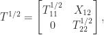
where 


edit private/sqrtm_tri at the MATLAB prompt. For more on this recursive scheme for computing square roots of triangular matrices see Blocked Schur Algorithms for Computing the Matrix Square Root (2013) by Deadman, Higham and Ralha.
The sqrtm in MATLAB 2015b includes two further refinements.
- For real matrices it uses the real Schur form, which means that all computations are carried out in real arithmetic, giving a speed advantage and ensuring that the result will not be contaminated by imaginary parts at the roundoff level.
- It estimates the 1-norm condition number of the matrix square root instead of the 2-norm condition number, so exploits the normest1 function.
Finally, I note that the product of two triangular matrices is also not a level-3 BLAS routine, yet again it is needed in matrix function codes. A proposal for it to be included in the Intel Math Kernel Library was made recently by Peter Kandolf, and I strongly support the proposal.
