Bfloat16 is a floating-point number format proposed by Google. The name stands for “Brain Floating Point Format” and it originates from the Google Brain artificial intelligence research group at Google.
Bfloat16 is a 16-bit, base 2 storage format that allocates 8 bits for the significand and 8 bits for the exponent. It contrasts with the IEEE fp16 (half precision) format, which allocates 11 bits for the significand but only 5 bits for the exponent. In both cases the implicit leading bit of the significand is not stored, hence the “+1” in this diagram:

The motivation for bfloat16, with its large exponent range, was that “neural networks are far more sensitive to the size of the exponent than that of the mantissa” (Wang and Kanwar, 2019).
Bfloat16 uses the same number of bits for the exponent as the IEEE fp32 (single precision) format. This makes conversion between fp32 and bfloat16 easy (the exponent is kept unchanged and the significand is rounded or truncated from 24 bits to 8) and the possibility of overflow in the conversion is largely avoided. Overflow can still happen, though (depending on the rounding mode): the significand of fp32 is longer, so the largest fp32 number exceeds the largest bfloat16 number, as can be seen in the following table. Here, the precision of the arithmetic is measured by the unit roundoff, which is 

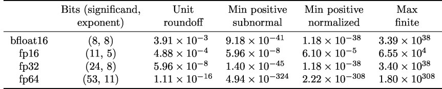
Note that although the table shows the minimum positive subnormal number for bfloat16, current implementations of bfloat16 do not appear to support subnormal numbers (this is not always clear from the documentation).
As the unit roundoff values in the table show, bfloat16 numbers have the equivalent of about three decimal digits of precision, which is very low compared with the eight and sixteen digits, respectively, of fp32 and fp64 (double precision).
The next table gives the number of numbers in the bfloat16, fp16, and fp32 systems. It shows that the bfloat16 number system is very small compared with fp32, containing only about 65,000 numbers.

The spacing of the bfloat16 numbers is large far from 1. For example, 65280, 65536, and 66048 are three consecutive bfloat16 numbers.
At the time of writing, bfloat16 is available, or announced, on four platforms or architectures.
- The Google Tensor Processing Units (TPUs, versions 2 and 3) use bfloat16 within the matrix multiplication units. In version 3 of the TPU the matrix multiplication units carry out the multiplication of 128-by-128 matrices.
- The NVIDIA A100 GPU, based on the NVIDIA Ampere architecture, supports bfloat16 in its tensor cores through block fused multiply-adds (FMAs)
with 8-by-8
and 8-by-4
.
- Intel has published a specification for bfloat16 and how it intends to implement it in hardware. The specification includes an FMA unit that takes as input two bfloat16 numbers
and
and an fp32 number
and computes
at fp32 precision, returning an fp32 number.
- The Arm A64 instruction set supports bfloat16. In particular, it includes a block FMA
The pros and cons of bfloat16 arithmetic versus IEEE fp16 arithmetic are
- bfloat16 has about one less (roughly three versus four) digit of equivalent decimal precision than fp16,
- bfloat16 has a much wider range than fp16, and
- current bfloat16 implementations do not support subnormal numbers, while fp16 does.
If you wish to experiment with bfloat16 but do not have access to hardware that supports it you will need to simulate it. In MATLAB this can be done with the chop function written by me and Srikara Pranesh.
References
This is a minimal set of references, which contain further useful references within.
- Arm A64 Instruction Set Architecture Armv8, for Armv8-A Architecture Profile, ARM Limited, 2019.
- Intel Corporation, BFLOAT16—Hardware Numerics Definition, 2018.
- IEEE Standard for Floating-Point Arithmetic, IEEE Std 754-2019 (Revision of IEEE 754-2008), The Institute of Electrical and Electronics Engineers, New York, 2019.
- NVIDIA Corporation, NVIDIA A100 Tensor Core GPU Architecture, 2020.
Related Blog Posts
- BFloat16 Processing for Neural Networks on Armv8-A by Nigel Stephens (2019)
- BFloat16: The Secret To High Performance on Cloud TPUs by Shibo Wang and Pankaj Kanwar (2019)
- A Multiprecision World (2017)
- Half Precision Arithmetic: fp16 Versus bfloat16 (2018)
- The Rise of Mixed Precision Arithmetic (2015)
- Simulating Low Precision Floating-Point Arithmetics in MATLAB (2020)
- What Is Floating-Point Arithmetic? (2020)
- What Is IEEE Standard Arithmetic? (2020)
This article is part of the “What Is” series, available from https://nhigham.com/category/what-is and in PDF form from the GitHub repository https://github.com/higham/what-is.


 .
. and
and  . It is easy to show that
  if
if  for general
 ![[A,B] = AB - BA](https://s0.wp.com/latex.php?latex=%5BA%2CB%5D+%3D+AB+-+BA&bg=ffffff&fg=222222&s=0&c=20201002) . For Hermitian
. For Hermitian  was proved independently by Golden and Thompson in 1965.
 , which is used in the scaling and squaring method for computing the matrix exponential.
 then
then

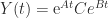
 , while the solution of the ODE in
  matrices
 .
. matrix
  such that
  .
. ), there are two square roots (which are equal if
  ), and they are real if and only if
  , depending on the matrix there can be no square roots, finitely many, or infinitely many. The matrix
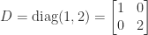
 . The identity matrix
 involutory matrices), including
  , the lower triangular matrix
![\begin{bmatrix} \cos \theta & \sin \theta \\ \sin \theta & -\cos \theta \end{bmatrix}, \quad \theta \in[0,2\pi]](https://s0.wp.com/latex.php?latex=%5Cbegin%7Bbmatrix%7D++++++%5Ccos+%5Ctheta++%26++%5Csin+%5Ctheta+%5C%5C++++++%5Csin+%5Ctheta++%26+-%5Ccos+%5Ctheta++++++%5Cend%7Bbmatrix%7D%2C+%5Cquad+%5Ctheta+%5Cin%5B0%2C2%5Cpi%5D+&bg=ffffff&fg=222222&s=0&c=20201002)
 . If
. If  above,
  .
. , where
  is orthogonal and
  is also symmetric positive definite.
 square roots, where
  such that
  is called a square root, but this is not the standard meaning.
 -matrices,
![G(\theta) = \begin{bmatrix} \cos \theta & \sin \theta \\ -\sin \theta & \cos \theta \end{bmatrix}, \quad \theta \in[0,2\pi],](https://s0.wp.com/latex.php?latex=G%28%5Ctheta%29+%3D+%5Cbegin%7Bbmatrix%7D++++++%5Ccos+%5Ctheta++%26++%5Csin+%5Ctheta+%5C%5C++++++-%5Csin+%5Ctheta++%26+%5Ccos+%5Ctheta++++++%5Cend%7Bbmatrix%7D%2C+%5Cquad+%5Ctheta+%5Cin%5B0%2C2%5Cpi%5D%2C+&bg=ffffff&fg=222222&s=0&c=20201002)
 radians clockwise. The natural square root of
  is
is  . For
. For  , this gives the square root
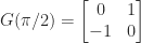
 th roots of stochastic matrices
![e\in [e_{\min},e_{\max}]](https://s0.wp.com/latex.php?latex=e%5Cin+%5Be_%7B%5Cmin%7D%2Ce_%7B%5Cmax%7D%5D&bg=ffffff&fg=222222&s=0&c=20201002) is the exponent. The significand
is the exponent. The significand  is an integer satisfying
  . Numbers with
  are called normalized. Subnormal numbers, for which
  and
and  , are supported.
 .
.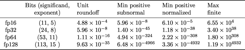 Fp32 (single precision) and fp64 (double precision) were in the 1985 standard; fp16 (half precision) and fp128 (quadruple precision) were introduced in 2008. Fp16 is defined only as a storage format, though it is widely used for computation.
 (usually written as inf in programing languages) as floating-point numbers: every arithmetic operation produces a number in the system. A NaN is generated by operations such as

 evaluates as
  when
when  .
.
 denotes the computed result. The standard also includes a fused multiply-add operation (FMA),
  . The definition requires it to be computed with just one rounding error, so that
  is the rounded version of
  , and hence satisfies
 ) and transcendental functions (
 ,
,  ,
,  ,
,  , etc.) and defines domains and special values for them, but these functions are not required.
 along with the error
  , for
, for  . These operations are useful for implementing compensated summation and other special high accuracy algorithms.
 is a finite subset of the real line comprising numbers of the form
 is the base,
  , and
, and  . The significand
 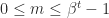 . Normalized numbers are those for which
  , and they have a unique representation. Subnormal numbers are those with
  and
and  is
is
 satisfies
  and
and  for normalized numbers.
 ,
,  , and
, and ![e \in [-1, 3]](https://s0.wp.com/latex.php?latex=e+%5Cin+%5B-1%2C+3%5D&bg=ffffff&fg=222222&s=0&c=20201002) .
.
 and
and  is
is  , which is called the machine epsilon. Note that
  .
. and the smallest normalized number, which is
  . The subnormal numbers fill this gap with numbers having the same spacing as those between
  , namely
  . The next diagram shows the complete set of nonnegative normalized and subnormal numbers in the toy system.
 is mapped into
  . If
. If  then
then  ; otherwise,
  and
and  then
then 
 .
. ,
,  ,
,  ,
,  , and
, and  are usually defined to return the correctly rounded exact result, so they satisfy
 , so all the numbers are equally spaced. In most scientific computations scale factors must be introduced in order to be able to represent the range of numbers occurring. Fixed-point arithmetic is mainly used on special purpose devices such as FPGAs and in embedded systems.
 to
to  , which can be described as rounding to three significant digits or two decimal places. Rounding does not change a number if it already has the requisite number of digits.
 ,
,  , or
, or  in floating-point arithmetic,
 and
and  and
and  , respectively, from
  to two significant digits, the result is
  with round to even and
  with round to odd.
 ,
,  ,
,  ,
,  ,
,  ,
,  with round to odd.
 or less and otherwise round up.
 rounds to
  . Similarly, with round towards minus infinity (or round down) we round to the next smaller number, so that
  .
. and round it up if
  . This is also known as chopping, or truncation.
 be the candidates for the result of rounding. We round up to
  with probability
  and down to
  with probability
  ; note that these probabilities sum to
  ), and round towards minus infinity (
 ). They show the number
 C and
C and  F round to
  C and
C and  F instead of
  C and
C and  F.
F. package
  is orthogonal and symmetric and we can choose the nonzero vector
  for any orthogonal (possibly non-random)
  and
and  . A random Householder matrix is not Haar distributed.
 has nonnegative diagonal elements. This construction requires
  flops.
 be an
be an  -vector of elements from the standard normal distribution and let
  be the Householder matrix that reduces
  , where
  is the first unit vector. Then
  is Haar distributed, where
  ,
,  , and
, and  . This construction expresses
  Householder matrices of growing effective dimension, and the product can be formed from right to left in
  flops. The MATLAB statement
  , where the elements of
  (where
  is symmetric positive semidefinite).
 .
. are column vectors with
  element
 is the mean of the elements in
  . If
. If  has nonzero diagonal elements then we can scale the diagonal to 1 to obtain the corresponding correlation matrix
 . The
. The  is the correlation between the variables
  .
.![[-1, 1]](https://s0.wp.com/latex.php?latex=%5B-1%2C+1%5D&bg=ffffff&fg=222222&s=0&c=20201002) .
.![[0,n]](https://s0.wp.com/latex.php?latex=%5B0%2Cn%5D&bg=ffffff&fg=222222&s=0&c=20201002) .
. (since the eigenvalues of a matrix sum to its trace).
 ,
,  ,
,  . The only value of
  and
and  that makes
  with every off-diagonal element equal to
  , illustrated for
  by
by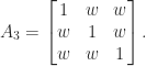
 .
. , so we solve the problem
 remain fixed. And we may want to weight some elements more than others, by using a weighted Frobenius norm. These are convex optimization problems and have a unique solution that can be computed using the alternating projections method (Higham, 2002) or a Newton algorithm (Qi and Sun, 2006; Borsdorf and Higham, 2010).
 matrix for some given
  , where
  and mutually orthogonal columns. For example,
![\left[\begin{array}{rrrr} 1 & 1 & 1 & 1\\ 1 & -1 & 1 & -1\\ 1 & 1 & -1 & -1\\ 1 & -1 & -1 & 1 \end{array}\right]](https://s0.wp.com/latex.php?latex=%5Cleft%5B%5Cbegin%7Barray%7D%7Brrrr%7D+++++++1+%26+1+%26+1+%26+1%5C%5C+++++++1+%26+-1+%26+1+%26+-1%5C%5C+++++++1+%26+1+%26+-1+%26+-1%5C%5C+++++++1+%26+-1+%26+-1+%26+1+%5Cend%7Barray%7D%5Cright%5D+&bg=ffffff&fg=222222&s=0&c=20201002)
 is that
  , so
, so  . It also follows that
  . Hadamard’s inequality states that for an
  , where
  is the
 ![\left[\begin{array}{rr} H & H\\ H & -H \end{array}\right].](https://s0.wp.com/latex.php?latex=%5Cleft%5B%5Cbegin%7Barray%7D%7Brr%7D++++++++++H+%26+H%5C%5C++++++++++H+%26+-H+++%5Cend%7Barray%7D%5Cright%5D.+&bg=ffffff&fg=222222&s=0&c=20201002)
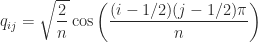
 for
for  . The MATLAB
 ![\left[\begin{array}{rrrrrrrrrrrr} {}+ & + & + & + & + & 1 & + & + & + & + & + & +\\ {}+ & - & + & - & + & + & + & - & - & - & + & -\\ {}+ & - & - & + & - & + & + & + & - & - & - & +\\ {}+ & + & - & - & + & - & + & + & + & - & - & -\\ {}+ & - & + & - & - & + & - & + & + & + & - & -\\ {}+ & - & - & + & - & - & + & - & + & + & + & -\\ {}+ & - & - & - & + & - & - & + & - & + & + & +\\ {}+ & + & - & - & - & + & - & - & + & - & + & +\\ {}+ & + & + & - & - & - & + & - & - & + & - & +\\ {}+ & + & + & + & - & - & - & + & - & - & + & -\\ {}+ & - & + & + & + & - & - & - & + & - & - & +\\ {}+ & + & - & + & + & + & - & - & - & + & - & - \end{array}\right].](https://s0.wp.com/latex.php?latex=%5Cleft%5B%5Cbegin%7Barray%7D%7Brrrrrrrrrrrr%7D+%7B%7D%2B+%26+%2B+%26+%2B+%26+%2B+%26+%2B+%26+1+%26+%2B+%26+%2B+%26+%2B+%26+%2B+%26+%2B+%26+%2B%5C%5C+%7B%7D%2B+%26+-+%26+%2B+%26+-+%26+%2B+%26+%2B+%26+%2B+%26+-+%26+-+%26+-+%26+%2B+%26+-%5C%5C+%7B%7D%2B+%26+-+%26+-+%26+%2B+%26+-+%26+%2B+%26+%2B+%26+%2B+%26+-+%26+-+%26+-+%26+%2B%5C%5C+%7B%7D%2B+%26+%2B+%26+-+%26+-+%26+%2B+%26+-+%26+%2B+%26+%2B+%26+%2B+%26+-+%26+-+%26+-%5C%5C+%7B%7D%2B+%26+-+%26+%2B+%26+-+%26+-+%26+%2B+%26+-+%26+%2B+%26+%2B+%26+%2B+%26+-+%26+-%5C%5C+%7B%7D%2B+%26+-+%26+-+%26+%2B+%26+-+%26+-+%26+%2B+%26+-+%26+%2B+%26+%2B+%26+%2B+%26+-%5C%5C+%7B%7D%2B+%26+-+%26+-+%26+-+%26+%2B+%26+-+%26+-+%26+%2B+%26+-+%26+%2B+%26+%2B+%26+%2B%5C%5C+%7B%7D%2B+%26+%2B+%26+-+%26+-+%26+-+%26+%2B+%26+-+%26+-+%26+%2B+%26+-+%26+%2B+%26+%2B%5C%5C+%7B%7D%2B+%26+%2B+%26+%2B+%26+-+%26+-+%26+-+%26+%2B+%26+-+%26+-+%26+%2B+%26+-+%26+%2B%5C%5C+%7B%7D%2B+%26+%2B+%26+%2B+%26+%2B+%26+-+%26+-+%26+-+%26+%2B+%26+-+%26+-+%26+%2B+%26+-%5C%5C+%7B%7D%2B+%26+-+%26+%2B+%26+%2B+%26+%2B+%26+-+%26+-+%26+-+%26+%2B+%26+-+%26+-+%26+%2B%5C%5C+%7B%7D%2B+%26+%2B+%26+-+%26+%2B+%26+%2B+%26+%2B+%26+-+%26+-+%26+-+%26+%2B+%26+-+%26+-+%5Cend%7Barray%7D%5Cright%5D.+&bg=ffffff&fg=222222&s=0&c=20201002)
 and
and  .
.
 is
is 
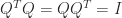 (the identity matrix). Equivalently,
  . The columns of an orthogonal matrix are orthonormal, that is, they have 2-norm (Euclidean length)
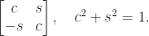
 and
and  for some
  for a
for a  vector
  , such a matrix has the form
 Householder reflector corresponding to
 ![v = [1,1,1,1]^T/2](https://s0.wp.com/latex.php?latex=v+%3D+%5B1%2C1%2C1%2C1%5D%5ET%2F2&bg=ffffff&fg=222222&s=0&c=20201002) :
:![\frac{1}{2} \left[\begin{array}{@{\mskip2mu}rrrr@{\mskip2mu}} 1 & -1 & -1 & -1\\ -1 & 1 & -1 & -1\\ -1 & -1 & 1 & -1\\ -1 & -1 & -1 & 1\\ \end{array}\right].](https://s0.wp.com/latex.php?latex=%5Cfrac%7B1%7D%7B2%7D+++++++++%5Cleft%5B%5Cbegin%7Barray%7D%7B%40%7B%5Cmskip2mu%7Drrrr%40%7B%5Cmskip2mu%7D%7D++++++++++++++++++++++++1+%26+++-1+%26+++-1+%26+++-1%5C%5C+++++++++++++++++++++++-1+%26++++1+%26+++-1+%26+++-1%5C%5C+++++++++++++++++++++++-1+%26+++-1+%26++++1+%26+++-1%5C%5C+++++++++++++++++++++++-1+%26+++-1+%26+++-1+%26++++1%5C%5C++++++++%5Cend%7Barray%7D%5Cright%5D.+&bg=ffffff&fg=222222&s=0&c=20201002)

 for any vector
  .
. is skew-symmetric (
 ) then
  (the matrix exponential) is orthogonal and the Cayley transform
  is orthogonal as long as
  , where
  is the conjugate transpose of