The latest release of MATLAB, R2016b, contains a feature called implicit expansion, which is an extension of the scalar expansion that has been part of MATLAB for many years. Scalar expansion is illustrated by
>> A = spiral(2), B = A - 1
A =
     1     2
     4     3
B =
     0     1
     3     2
Here, MATLAB subtracts 1 from every element of A, which is equivalent to expanding the scalar 1 into a matrix of ones then subtracting that matrix from A.
Implicit expansion takes this idea further by expanding vectors:
>> A = ones(2), B = A + [1 5]
A =
     1     1
     1     1
B =
     2     6
     2     6
Here, the result is the same as if the row vector was replicated along the first dimension to produce the matrix [1 5; 1 5] then that matrix was added to ones(2). In the next example a column vector is added and the replication is across the columns:
>> A = ones(2) + [1 5]'
A =
     2     2
     6     6
Implicit expansion also works with multidimensional arrays, though we will focus here on matrices and vectors.
So MATLAB now treats “matrix plus vector” as a legal operation. This is a controversial change, as it means that MATLAB now allows computations that are undefined in linear algebra.
Why have MathWorks made this change? A clue is in the R2016b Release Notes, which say
For example, you can calculate the mean of each column in a matrix A, then subtract the vector of mean values from each column with A - mean(A).
This suggests that the motivation is, at least partly, to simplify the coding of manipulations that are common in data science.
Implicit expansion can also be achieved with the function bsxfun that was introduced in release R2007a, though I suspect that few MATLAB users have heard of this function:
>> A = [1 4; 3 2], bsxfun(@minus,A,mean(A))
A =
     1     4
     3     2
ans =
    -1     1
     1    -1

>> A - mean(A)
ans =
    -1     1
     1    -1
Prior to the introduction of bsxfun, the repmat function could be used to explicitly carry out the expansion, though less efficiently and less elegantly:
>> A - repmat(mean(A),size(A,1),1)
ans =
    -1     1
     1    -1
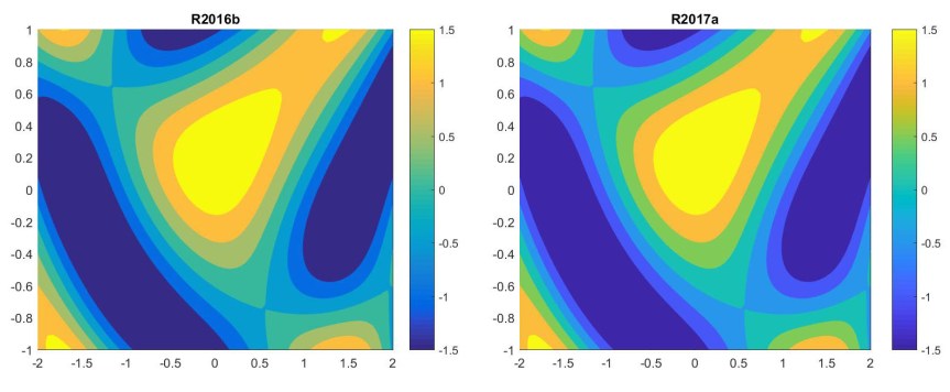
An application where the new functionality is particularly attractive is multiplication by a diagonal matrix.
>> format short e
>> A = ones(3); d = [1 1e-4 1e-8];
>> A.*d  %  A*diag(d)
ans =
   1.0000e+00   1.0000e-04   1.0000e-08
   1.0000e+00   1.0000e-04   1.0000e-08
   1.0000e+00   1.0000e-04   1.0000e-08
>> A.*d' % diag(d)*A
ans =
   1.0000e+00   1.0000e+00   1.0000e+00
   1.0000e-04   1.0000e-04   1.0000e-04
   1.0000e-08   1.0000e-08   1.0000e-08
The .* expressions are faster than forming and multiplying by diag(d) (as is the syntax bsxfun(@times,A,d)). We can even multiply with the inverse of diag(d) with
>> A./d
ans =
           1       10000   100000000
           1       10000   100000000
           1       10000   100000000
It is now possible to add a column vector to a row vector, or to subtract them:
>> d = (1:3)'; d - d'
ans =
     0    -1    -2
     1     0    -1
     2     1     0
This usage allows very short expressions for forming the Hilbert matrix and Cauchy matrices (look at the source code for hilb.m with type hilb or edit hilb).
The max and min functions support implicit expansion, so an elegant way to form the matrix  with
with  element
  is with
d = (1:n); A = min(d,d');
and this is precisely what gallery('minij',n) now does.
Another function that can benefit from implicit expansion is vander, which forms a Vandermonde matrix. Currently the function forms the matrix in three lines, with calls to repmat and cumprod. Instead we can do it as follows, in a formula that is closer to the mathematical definition and hence easier to check.
A = (v(:) .^ (n-1:-1:0)')'; % Equivalent to A = vander(v)
The latter code is, however, slower than the current vander for large dimensions, presumably because exponentiating each element independently is slower than using repeated multiplication.
An obvious objection to implicit expansion is that it could cause havoc in linear algebra courses, where students will be able to carry out operations that the instructor and textbook have said are not allowed. Moreover, it will allow programs with certain mistyped expressions to run that would previously have generated an error, making debugging more difficult.
I can see several responses to this objection. First, MATLAB was already inconsistent with linear algebra in its scalar expansion. When a mathematician writes (with a common abuse of notation)  , with a scalar
  , he or she usually means
  and not
  with
with  the matrix of ones.
Second, I have been using the prerelease version of R2016b for a few months, while working on the third edition of MATLAB Guide, and have not encountered any problems caused by implicit expansion—either with existing codes or with new code that I have written.
A third point in favour of implicit expansion is that it is particularly compelling with elementwise operations (those beginning with a dot), as the multiplication by a diagonal matrix above illustrates, and since such operations are not a part of linear algebra confusion is less likely.
Finally, it is worth noting that implicit expansion fits into the MATLAB philosophy of “useful defaults” or “doing the right thing”, whereby MATLAB makes sensible choices when a user’s request is arguably invalid or not fully specified. This is present in the many functions that have optional arguments. But it can also be seen in examples such as
% No figure is open and no parallel pool is running.
>> close         % Close figure.
>> delete(gcp)   % Shut down parallel pool.
where no error is generated even though there is no figure to close or parallel pool to shut down.
I suspect that people’s reactions to implicit expansion will be polarized: they will either be horrified or will regard it as natural and useful. Now that I have had time to get used to the concept—and especially now that I have seen the benefits both for clarity of code (the minij matrix) and for speed (multiplication by a diagonal matrix)—I like it. It will be interesting to see the community’s reaction.


 ) is standard notation for a perturbation of the matrix
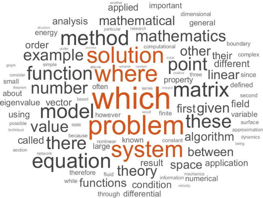
 Wordle removes certain stop words (common but unimportant words) that

 can be represented by a pair of double precision numbers
  , where
  and
and  and
and  represent the leading and trailing significant digits of
  can be written
  , which involves four double precision multiplications and three double precision additions. We can therefore expect quadruple precision multiplication to be at least seven times slower than double precision multiplication. Almost all available implementations of quadruple precision arithmetic are in software (an exception is provided by the