What Is a Matrix?

A matrix is a rectangular array of numbers on which certain algebraic operations are defined. Matrices provide a convenient way of encapsulating many numbers in a single object and manipulating those numbers in useful ways.

An $m \times n$ matrix has $m$ rows and $n$ columns and $m$ and $n$ are called the dimensions of the matrix. A matrix is square if it has the same number of rows and columns, otherwise it is rectangular.

An example of a square matrix is

$\begin{bmatrix} 1 & 1 & 1 & 1\\ 1 & 2 & 3 & 4\\ 1 & 3 & 6 & 10\\ 1 & 4 & 10 & 20 \end{bmatrix}.$

This matrix is symmetric: $a_{ij} = a_{ji}$ for all $i$ and $j$ , where $a_{ij}$ denotes the entry at the intersection of row $i$ and column $j$ . Matrices are written either with square brackets, as in this example, or round brackets (parentheses).

Addition of matrices of the same dimensions is defined in the obvious way: by adding the corresponding entries.

Multiplication of matrices requires the inner dimensions to match. The product of an $m \times p$ matrix $A$ and an $p\times n$ matrix $B$ is an $m\times n$ matrix $C = AB$ defined by the formula

$c_{ij} = \displaystyle\sum_{k=1}^p a_{ik}b_{kj}, \quad 1 \le i \le m, \quad 1 \le j \le n.$

When $m = n$ , both $AB$ and $BA$ are defined, but they are generally unequal: matrix multiplication is not commutative.

The inverse of a square matrix $A$ is a matrix $X$ such that $AX = XA = I$ , where $I$ is the identity matrix, which has ones on the main diagonal (that is, in the $(i,i)$ position for all $i$ ) and zeros off the diagonal. For rectangular matrices various notions of generalized inverse exist.

The transpose of an $m \times n$ matrix $A$ , written $A^T$ , is the $n \times m$ matrix whose $(i,j)$ entry is $a_{ji}$ . For a complex matrix, the conjugate transpose, written $A^*$ or $A^H$ , has $(i,j)$ entry $\overline{a}_{ji}$ .

In linear algebra, a matrix represents a linear transformation between two vector spaces in terms of particular bases for each space.

Vectors and scalars are special cases of matrices: column vectors are $n\times 1$ , row vectors are $1\times n$ , and scalars are $1\times1$ .

Many programming languages and problem solving environments support arrays. It is important to note that operations on arrays are typically defined componentwise, so that, for example, multiplying two arrays multiplies the corresponding pairs of entries, which is not the same as matrix multiplication. The quintessential programming environment for matrices is MATLAB, in which a matrix is the core data type.

It is possible to give meaning to a matrix with one or both dimensions zero. MATLAB supports such empty matrices. Matrix multiplication generalizes in a natural way to allow empty dimensions:

>> A = zeros(0,2)*zeros(2,3)
A =
0x3 empty double matrix

>> A = zeros(2,0)*zeros(0,3)
A =
0     0     0
0     0     0

In linear algebra and numerical analysis, matrices are usually written with a capital letter and vectors with a lower case letter. In some contexts matrices are distinguished by boldface.

The term matrix was coined by James Joseph Sylvester in 1850. Arthur Cayley was the first to define matrix algebra, in 1858.

References

Arthur Cayley, A Memoir on the Theory of Matrices, Philos. Trans. Roy. Soc. London 148, 17–37, 1858.
Nicholas J. Higham, Sylvester’s Influence on Applied Mathematics, Mathematics Today 50, 202–206, 2014. A version of the article with an extended bibliography containing additional historical references is available as a MIMS EPrint.
Roger A. Horn and Charles R. Johnson, Matrix Analysis, second edition, Cambridge University Press, 2013. My review of the second edition.

Update of Catalogue of Software for Matrix Functions

Edvin Hopkins and I have updated to version 3.0 the catalogue of software for matrix functions that we originally produced in 2014 and updated in 2016. It covers what is available in various languages (C++, Fortran, Java, Julia, Python, Rust), problem solving environments (GNU Octave, Maple, Mathematica, MATLAB and associated toolboxes, R, Scilab), and libraries (Armadillo, GNU Scientific Library, NAG Library, SLEPc, SLICOT).

Here are some highlights of changes in the last four years that are reflected in the new version.

Several new MATLAB third-party functions have been written, by various authors, notably for $f(A)b$ and for arbitrary precision evaluation of the exponential and logarithm.
Matrix function support in Julia has been expanded.
Armadillo, Rust, SLEPc, and Tensorflow are included in new entries.

In addition, all URLs and references have been updated.

Suggestions for inclusion in a future revision are welcome.

What Is Backward Error?

Backward error is a measure of error associated with an approximate solution to a problem. Whereas the forward error is the distance between the approximate and true solutions, the backward error is how much the data must be perturbed to produce the approximate solution.

For a function $f$ from $\mathbb{R}^n$ to $\mathbb{R}^n$ and an approximation $y$ to $f(x)$ , the backward error in $y$ is the smallest $\Delta x$ such that $y = f(x+\Delta x)$ , for some appropriate measure of size. There can be many $\Delta x$ satisfying this equation, so the backward error is the solution to a minimization problem. Using a vector norm and measuring perturbations in a relative sense, we can define the backward error in $y$ as

$\eta(y) = \min\{ \, \epsilon: y = f(x+\Delta x), \; \|\Delta x\| \le \epsilon \|x\| \,\}.$

In the following figure the solid lines denote exact mappings and the dashed line shows the mapping that was actually computed.

Usually, but not always, the errors in question are rounding errors, but backward error can also be a useful way to characterize truncation errors (for example in deriving algorithms based on Padé approximation for computing matrix functions).

As an example, for the inner product $u^Tv$ of two vectors the backward error of an approximation $w$ can be defined as

$\eta(w) = \min \{\, \epsilon: w = (u + \Delta u)^Tv,\; \|\Delta u\|_2 \le \epsilon \|u\|_2 \,\},$

where $\|u\|_2 = (u^Tu)^{1/2}$ . It can be shown that

$\eta(w) = \displaystyle\frac{ |w - u^Tv| }{ \|u\|_2 \|v\|_2 }.$

The definition of $\eta(w)$ is clearly unsymmetric in that $u$ is perturbed but $v$ is not. If $v$ is perturbed instead of $u$ then the same formula is obtained. If both $u$ and $v$ are perturbed then the constraint in the definition of $\eta(w)$ becomes nonlinear in $\Delta u$ and $\Delta v$ and no explicit formula is available for $\eta(w)$ .

For some problems a backward error may not exist. An example is computation of the outer product $A = uv^T$ of two $n$ -vectors, which has rank 1. In floating-point arithmetic the computed matrix $\widehat{A}$ is unlikely to be of rank 1, so $\widehat{A} = (u + \Delta u)(v + \Delta v)^T$ is not in general possible for any $\Delta u$ and $\Delta v$ . In this situation one can consider a mixed backward–forward error that perturbs $\widehat{A}$ as well as $u$ and $v$ .

Backward error analysis refers to rounding error analysis in which a bound is obtained for a suitably defined backward error. If the backward error can be shown to be small then $y$ is the solution to a nearby problem. Indeed, if the backward error can be shown to be of the same size as any uncertainties in the data then $y$ is as good a solution as can be expected.

Backward error analysis was developed and popularized by James Wilkinson in the 1950s and 1960s. He first used it in the context of computing zeros of polynomials, but the method’s biggest successes came when he applied it to linear algebra computations.

Backward error analysis has also been used in the context of the numerical solution of differential equations, where it is used in different forms known as defect control and shadowing.

The forward error of $y\approx f(x)$ is bounded in terms of the backward error $\eta(y)$ by

$\displaystyle\frac{\|y - f(x)\|}{\|f\|} \le \mathrm{cond}(f,x) \eta(y) + O(\eta(y))^2,$

in view of the definition of condition number. Consequently, we have the rule of thumb that

$\mbox{forward error} \lesssim \mbox{condition number}\times \mbox{backward error}.$

References

This is a minimal set of references, which contain further useful references within.

Robert M. Corless and Nicolas Fillion, A Graduate Introduction to Numerical Methods from the Viewpoint of Backward Error Analysis, Springer, 2013.
Wayne Hayes and Kenneth R. Jackson, A survey of shadowing methods for numerical solutions of ordinary differential equations, Appl. Numer. Math. 53, 299–321, 2005.
Nicholas J. Higham, Accuracy and Stability of Numerical Algorithms, second edition, Society for Industrial and Applied Mathematics, Philadelphia, PA, USA, 2002.

What Is a Condition Number?

A condition number of a problem measures the sensitivity of the solution to small perturbations in the input data. The condition number depends on the problem and the input data, on the norm used to measure size, and on whether perturbations are measured in an absolute or a relative sense. The problem is defined by a function, which may be known explicitly or may be only implicitly defined (as when the problem is to solve an equation).

The most well known example of a condition number is the condition number of a nonsingular square matrix $A$ , which is $\kappa(A) = \|A\| \|A^{-1}\|$ . More correctly, this is the condition number with respect to inversion, because a relative change to $A$ of norm $\epsilon$ can change $A^{-1}$ by a relative amount as much as, but no more than, about $\kappa(A)\epsilon$ for small $\epsilon$ . The same quantity $\kappa(A)$ is also the condition number for a linear system $Ax = b$ (exactly if $A$ is the data, but only approximately if both $A$ and $b$ are the data).

It is easy to see that $\kappa(A) \ge 1$ for any norm for which $\|I\| = 1$ (most common norms, but not the Frobenius norm, have this property) and that $\kappa(A)$ tends to infinity as $A$ tends to singularity.

A general definition of (relative) condition number, for a function $f$ from $\mathbb{R}^n$ to $\mathbb{R}^n$ , is

$\mathrm{cond}(f,x) = \lim_{\epsilon\to0} \displaystyle\sup_{\|\Delta x\| \le \epsilon \|x\|} \displaystyle\frac{\|f(x+\Delta x) - f(x)\|}{\epsilon\|f(x)\|}.$

Taking a small, nonzero $\epsilon$ , we have

$\displaystyle\frac{\|f(x+\Delta x) - f(x)\|}{\|f(x)\|} \lesssim \mathrm{cond}(f,x) \displaystyle\frac{\|\Delta x\|}{\|x\|}$

for small $\|\Delta x\|$ , with approximate equality for some $\Delta x$ .

An explicit expression for $\mathrm{cond}(f,x)$ can be given in terms of the Jacobian matrix, $J(x) = (\partial f_i/\partial x_j)$ :

$\mathrm{cond}(f,x) = \displaystyle\frac{ \|x\| \| J(x) \| }{ \| f(x) \|}.$

We give two examples.

If $f$ is a scalar function then $J(x) = f'(x)$ , so $\mathrm{cond}(f,x) = |xf'(x)/f(x)|$ . Hence, for example, $\mathrm{cond}(\log,x) = 1/|\log x|$ .
If $z$ is a simple (non-repeated) root of the polynomial $p(t) = a_n t^n + \cdots + a_1 t + a_0$ then the data is the vector of coefficients $a = [a_n,\dots,a_0]^T$ . It can be shown that the condition number of the root $z$ is, for the $\infty$ -norm,
$\mathrm{cond}(z,a) = \displaystyle\frac{ \max_i |a_i| \sum_{i=0}^n |z|^i } { |z p'(z)| }.$

A general theory of condition numbers was developed by Rice (1966).

A problem is said to be well conditioned if the condition number is small and ill conditioned if the condition number is large. The meaning of “small” and “large” depends on the problem and the context. This diagram illustrates a well-conditioned function $f$ : small changes in $x$ produce small changes in $f$ .

The next diagram depicts an ill-conditioned function $f$ : small changes in $x$ can produce large changes in $f$ (but do not necessarily do so, as the closeness of $f(x_2)$ and $f(x_3)$ illustrates).

Here are a few key points about condition numbers.

Even though an explicit expression may be available for it, computing $\mathrm{cond}(f,x)$ is usually as expensive as computing $f(x)$ , so a lot of research has focused on obtaining inexpensive estimates of the condition number or bounds for it.
While $\kappa(A) \ge 1$ , it is not true for all functions that $\mathrm{cond}(f,x)$ is bounded below by $1$ .
For a range of functions that includes the matrix inverse, matrix eigenvalues, and a root of a polynomial, it is known that the condition number is the reciprocal of the relative distance to the nearest singular problem (one with an infinite condition number).
As the condition number is itself a function, one can ask: What is the condition number of the condition number? For a variety of problems, including those mentioned in the previous point, the condition number of the condition number is (approximately) the condition number!

References

This is a minimal set of references, which contain further useful references within.

James W. Demmel, On Condition numbers and the distance to the nearest ill-posed problem, Numer. Math. 51, 251–289, 1987.
Desmond J.Higham, Condition numbers and their condition numbers, Linear Algebra Appl. 214, 193–213, 1995.
Nicholas J. Higham, Accuracy and Stability of Numerical Algorithms, second edition, Society for Industrial and Applied Mathematics, Philadelphia, PA, USA, 2002.
Nicholas J. Higham, Functions of Matrices: Theory and Computation, Society for Industrial and Applied Mathematics, Philadelphia, PA, USA, 2008. (Chapter 3).
Nicholas J. Higham and Samuel D. Relton, Higher order Fréchet derivatives of matrix functions and the level- $2$ condition number, SIAM J. Matrix Anal. Appl. 35(3), 1019–1037, 2014.
John R. Rice, A theory of condition, SIAM J. Numer. Anal. 3(2), 287–310, 1966.

“What Is” Series

I am starting a series of “What Is” posts. These will give brief descriptions of important concepts in numerical analysis and related areas, with a focus on topics that arise in my research. I will try to adhere to the following criteria.

The posts are no more than two or three screenfuls (about 500 words).
The posts contain a minimum of mathematical symbols, equations, and citations.
The posts are accessible to upper level undergraduate students in any mathematically oriented subject.
The list of references given for further reading is very small and concentrates on those that are broad, readable, and contain further references to the literature.

I will make PDF versions (from $\LaTeX$ ) of the posts available on GitHub in the repository What-Is. These are much better for printing. They contain hyperlinks, which will be clickable in the PDF but not visible in a printout.

I will be happy to receive suggestions for topics to cover.

From 2002–2019 the Notices of the American Mathematical Society published a “What Is …” series of articles, latterly in the Graduate Student section. An index of the articles is available here. Those articles are almost exclusively on pure mathematics and I don’t anticipate much, if any, overlap with my series.

Handbook of Writing for the Mathematical Sciences, Third Edition

The third edition of Handbook of Writing for the Mathematical Sciences was published by SIAM in January 2020. It is SIAM’s fourth best selling book of all time if sales for the first edition (1993) and second edition (1998) are combined, and it is in my top ten most cited outputs. As well as being used by individuals from students to faculty, it is a course text on transferable skills modules in many mathematics departments. A number of publishers cite the book as a reference for recommended style—see, for example, the AMS Author Handbook, the SIAM Style Manual and, outside mathematics and computing, the Chicago Manual of Style.

Parts of the second edition were becoming out of date, as they didn’t reflect recent developments in publishing (open access publishing, DOIs, ORCID, etc.) or workflow (including modern LaTeX packages, version control, and markup languages). I’ve also learned a lot more about writing over the last twenty years.

I made a variety of improvements for the third edition. I reorganized the material in a way that is more logical and makes the book easier to use for reference. I also improved the design and formatting and checked and updated all the references.

I removed content that was outdated or is now unnecessary. For example, nowadays there is no need to talk about submitting a hard copy manuscript, or one not written in LaTeX, to a publisher. I removed the 20-page appendix Winners of Prizes for Expository Writing, since the contents can now be found on the web, and likewise for the appendix listing addresses of mathematical organizations.

I also added a substantial amount of new material. Here are some of the more notable changes.

A new chapter Workflow discusses how to organize and automate the many tasks involved in writing. With the increased role of computers in writing and the volume of digital material we produce it is important that we make efficient use of text editors, markup languages, tools for manipulating plain text, spellcheckers, version control, and much more.
The chapter on $\LaTeX$ has been greatly expanded, reflecting both the many new and useful packages and my improved knowledge of typesetting.
I used the enumitem $\LaTeX$ package to format all numbered and bulleted lists. This results in more concise lists that make better use of the page, as explained in this blog post.
I wrote a new chapter on indexing at the same time as I was reading the literature on indexing and making an improved index for the book. Indexing is an interesting task, but most of us do it only occasionally so it is hard to become proficient. This is my best index yet, and the indexing chapter explains pretty much everything I’ve learned abut the topic.
Since the second edition I have changed my mind about how to typeset tables. I am now a convert to minimizing the use of rules and to using the booktabs $\LaTeX$ package, as explained in this blog post.
The chapter Writing a Talk now illustrates the use of the Beamer $\LaTeX$ package.
The book uses color for syntax highlighted $\LaTeX$ listings and examples of slides.
Sidebars in gray boxes give brief diversions on topics related to the text, including several on “Publication Peculiarities”.
An expanded chapter English Usage includes new sections on Zombie Nouns; Double Negatives; Serial, or Oxford, Comma; and Split Infinitives.
There are new chapters on Writing a Blog Post; Refereeing and Reviewing; Writing a Book; and, as discussed above, Preparing an Index and Workflow.
The bibliography now uses the backref $\LaTeX$ package to point back to the pages on which entries are cited, hence I removed the author index.
As well as updating the bibliography I have added DOIs and URL links, which can be found in the online version of the bibliography in bbl and PDF form, which is available from the book’s website.

At 353 pages, and allowing for the appendices removed and the more efficient formatting, the third edition is over 30 percent longer than the second edition.

As always, working with the SIAM staff on the book was a pleasure. A special thanks goes to Sam Clark of T&T Productions, who copy edited the book. Sam, with whom I have worked on two previous book projects, not only edited for SIAM style but found a large number of improvements to the text and showed me some things I did not know about $\LaTeX$ .

SIAM News has published an interview with me about the book and mathematical writing and publishing.

Here is a word cloud for the book, generated in MATLAB using the wordcloud function, based on words of 6 or more characters.

Accurately Computing the Softmax Function

The softmax function takes as input an $n$ -vector $x$ and returns a vector $g(x)$ with elements

$g_j(x) = \displaystyle\frac{\mathrm{e}^{x_j}}{\sum_{i=1}^n \mathrm{e}^{x_i}}, \quad j=1\colon n,$

The elements of $g$ are all between $0$ and $1$ and they sum to 1, so $g$ can be regarded as a vector of probabilities. Softmax is a key function in machine learning algorithms.

Softmax is the gradient vector of the log-sum-exp function

$f(x) = \displaystyle\log \sum_{i=1}^n \mathrm{e}^{x_i}.$

This function is an approximation to the largest element, $x_{\max} = \max_i x_i$ of the vector $x$ , as it lies between $x_{\max}$ and $x_{\max} + \log n$ .

A problem with numerical evaluation of log-sum-exp and softmax is that overflow is likely even for quite modest values of $x_i$ because of the exponentials, even though $g(x)$ cannot overflow and $f(x)$ is very unlikely to do so.

A standard solution it to incorporate a shift, $a$ , and use the formulas

$f(x) = a + \displaystyle\log \sum_{i=1}^n \mathrm{e}^{x_i-a}, \hspace*{4.5cm}(1)$

and

$g_j(x) = \displaystyle\frac{\mathrm{e}^{x_j-a}}{\sum_{i=1}^n \mathrm{e}^{x_i-a}}, \quad j=1\colon n, \hspace*{3.3cm}(2)$

where $a$ is usually set to $x_{\max}$ .

Another formula for softmax is obtained by moving the denominator into the numerator:

$g_j(x) = \exp\left(x_j - a - \log\displaystyle\sum_{i=1}^n\mathrm{e}^{x_i -a}\right). \hspace*{2cm}(3)$

This formulas is used in various codes, including in the SciPy 1.4.1 function softmax.

How accurate are these formulas when evaluated in floating-point arithmetic? To my knowledge, this question has not been addressed in the literature, but it is particularly important given the growing use of low precision arithmetic in machine learning. Two questions arise. First, is there any difference between the accuracy of the formulas (2) and (3) for $g_j(x)$ ? Second, in (1) and (3), $a$ is added to a nonnegative log term, so when $a = x_{\max}$ is negative can there be damaging subtractive cancellation?

In a recent EPrint with Pierre Blanchard and Des Higham I have investigated these questions using rounding error analysis and analysis of the conditioning of the log-sum-exp and softmax problems. In a nutshell, our findings are that while cancellation can happen, it is not a problem: the shifted formulas (1) and (2) can be safely used.

However, the alternative softmax formula (3) is not recommended, as its rounding error bounds are larger than for (2) and we have found it to produce larger errors in practice.

Here is an example from training an artificial neural network using the MATLAB Deep Learning Toolbox. The network is trained to classify handwritten digits from the widely used MNIST data set. The following figure shows the sum of the computed elements of the softmax vector $g(x)$ for 2000 vectors extracted from the training data, where $g(x)$ was computed in IEEE half precision arithmetic. The sum should be 1. The red circles are for formula (2) and the blue crosses are for the division-free formula (3). Clearly, (2) gives a better approximation to a vector of probabilities (in the sense of respecting the constraint that probabilities sum to unity); the actual errors in each vector component are also smaller for (2).

Lists in LaTeX with the enumitem Package

$\LaTeX$ provides the enumerate and itemize environments for numbered and itemized (usually bulleted) lists, respectively. Various package are available that provide more customizable list environments. While preparing the third edition of Handbook of Writing for the Mathematical Sciences I came across the enumitem package and ended up using it to typeset lists throughout the book.

As well as allowing all the customizations I could possibly need, enumitem has two very useful built-in options. By default, $\LaTeX$ lists contain quite a lot of vertical space. The nosep option, used as in

\begin{itemize}[nosep]
...
\end{itemize}

(and similarly for enumerate) removes vertical spaces in the list. The wide option, used as in

\begin{itemize}[wide]
...
\end{itemize}

produces lists whose entries have zero indentation on the second and subsequent lines. Both options save space and look better to my eye, especially for a book. They can be combined by specifying [wide,nosep].

An example of a customization possible with enumitem is

\begin{enumerate}[label=X\arabic*.,ref=X\arabic*]
\item\label{item1}
...
\end{enumerate}

This enumerated list has labels X1, X2, etc., and a reference such as “see \ref{item1}" reproduces the label: “see X1”.

Description environments can also be customized (I use these very little).

For examples of the above customizations see the LaTeX file and PDF output (shown to the right) in my enumitem_demo repository on GitHub.

These examples barely scratch the surface of the customizations that enumitem makes possible. Consult the manual for full details.

For guidance on how to punctuate lists see Handbook of Writing for the Mathematical Sciences (section 3.26) or my blog post Punctuating Lists.

A Mathematician Looks at the Collins English Dictionary

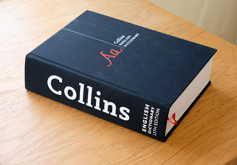
I have several dictionaries on my shelf, among which is a well-thumbed Collins English Dictionary (third edition, 1991). Earlier this year I acquired the thirteenth edition (2018). At 26.5cm high, 20cm wide, and 6.5cm deep, and weighing approximately 2.5kg, it’s an imposing tome. It’s printed on thin paper with minimal show-through and in a specially designed font (Collins Fedra) that is very legible.

The thirteenth edition, which I will abbreviate to CED13, is a wonderful acquisition for any dictionary lover. It has a wide coverage, including

new words such as micromort (“a unit of risk equal to a one-in-a million chance of dying”),
obscure words such as compotation (“the act of drinking together in a company”), and
a wide selection of proper nouns, including my home town Eccles and, somewhat unexpectedly, Laurel and Hardy and Torvill and Dean (Olympic ice dance champions, 1984).

It has no appendices on English usage, mathematical symbols, chemical elements, etc., as are found in many dictionaries—which is fine with me as I rarely use them.

I decided to take a close look at some of the mathematical words in the CED.

“determinant n maths: a square array of elements that represents the sum of certain products of these elements, used to solve simultaneous equations, in vector studies, etc.”

This definition has two problems. First, a determinant is the sum, not something that represents the sum. Of, course, one will find in some textbooks statements such as “swapping two rows of a determinant changes its sign”, but it’s odd that this informal usage of determinant as array is the only one mentioned. A second problem is that the determinant is not a sum of products: it is a signed sum of products and it is the permanent (not in this dictionary) that is obtained by taking all positive signs.

“matrix n maths a rectangular array of elements set out in rows and columns, used to facilitate the solution of problems, such as transformation of coordinates.”

A matrix is more than just an array: its key characteristic is that it has algebraic operations defined on it.

“rounding: n computing a process in which a number is approximated as the closest number that can be expressed using the number of bits or digits available.”

Rounding is not specifically a computing term—it’s more fundamentally a mathematical operation and predates computing. Bits are special cases of digits. And rounding does not have to be to the closest number: in some situations once needs to round to the next larger or smaller number.

“index n maths c a subscript or superscript to the right of a variable to express a set of variables, as in using $x_i$ for $x_1$ , $x_2$ , $x_3$ , etc”

An index does not (except maybe in informal usage) express a set, but rather identifies a member of a set.

“supercomputer n a powerful computer that can process large quantities of data of a similar type very quickly.”

Supercomputers do mathematical calculations (and are ranked on their speed in doing so), which is not apparent from this definition. I’m also not sure why “of a similar type” is necessary. The PC on which I am typing is a supercomputer according to this definition!

“integral n maths the limit of an increasingly large number of increasingly smaller quantities, related to the function that is being integrated (the integrand). The independent variables may be confined within certain limits (definite integral) or in the absence of limits (indefinite integral).”

This seems to be an attempt to state informally the Riemann sum definition of definite integration. Sadly, it’s technically incomplete and sure to baffle anyone who doesn’t already know about Riemann sums. It would have been much better to simply say that integration is the inverse of differentiation. The second sentence is grammatically incorrect.

“fractal maths n a figure or surface generated by successive subdivisions of a simpler polygon or polyhedron, according to some iterative process.”

Surely any definition should mention fractional dimension and self-similarity? This definition excludes the fractal that is the boundary of the Mandelbrot set.

I’m not too surprised by these weaknesses, because in 1994 I wrote an article Which Dictionary for the Mathematical Scientist? (PDF file here) in which I evaluated several dictionaries (including CED3) from the point of view of their mathematical words and found problems such as those above in several of them.

Despite these criticisms, I very much like this dictionary and I use it as much as the other dictionaries on my desk. It is especially good on the computing side. I was pleased to see that my favourite editor, emacs, is included (though I’m not sure why it is not capitalized). Vi users will be sad to hear that Vi is not included. A good number of programming languages are present, including awk (uncapitalized), Java, and Javascript, but not, C++ (how would that be alphabetized?), Python, or R.

A particularly notable definition is

“flops or FLOPS n acronym for floating-point operations per second: used as a measure of computer processing power (in combination with a prefix): megaflops; gigaflops.”

This is much better than the Oxford English Dictionary’s definition of the singular flop as “a floating-point operation per second”. There are also entries for petaflop, “ $10^{15}$ floating-point operations a second”, and teraflop, “a thousand billion floating-point operations a second”. I just wish the latter definition contained “ $10^{12}$ “, because there is scope for misunderstanding because of the alternative meaning of a billion as a million million in the UK.

What Is a Matrix?

References

Related Blog Posts

Update of Catalogue of Software for Matrix Functions

What Is Backward Error?

References

Related Blog Posts

What Is a Condition Number?

References

Related Blog Posts

“What Is” Series

Handbook of Writing for the Mathematical Sciences, Third Edition

Accurately Computing the Softmax Function

Top Five Posts of 2019

Lists in LaTeX with the enumitem Package

A Mathematician Looks at the Collins English Dictionary

References

Related Blog Posts

Share this:

Share this:

References

Related Blog Posts

Share this:

References

Related Blog Posts

Share this:

Share this:

Share this:

Share this:

Share this:

Share this:

Share this: