July 2023 – Nick Higham

The pseudoinverse is an extension of the concept of the inverse of a nonsingular square matrix to singular matrices and rectangular matrices. It is one of many generalized inverses, but the one most useful in practice as it has a number of special properties.

The pseudoinverse of a matrix $A\in\mathbb{C}^{m\times n}$ is an $n \times m$ matrix $X$ that satisfies the Moore–Penrose conditions

$\notag \begin{array}{rcrc} \mathrm{(1)} & AXA = A, \; & \mathrm{(2)} & XAX=X,\\ \mathrm{(3)} & (AX)^* = AX, \; & \mathrm{(4)} & (XA)^* = XA. \end{array}$

Here, the superscript $*$ denotes the conjugate transpose. It can be shown that there is a unique $X$ satisfying these equations. The pseudoinverse is denoted by $A^+$ ; some authors write $A^\dagger$ .

The most important property of the pseudoinverse is that for any system of linear equations $Ax = b$ (overdetermined or underdetermined) $x = A^+b$ minimizes $\|Ax - b\|_2$ and has the minimum $2$ -norm over all minimizers. In other words, the pseudoinverse provides the minimum $2$ -norm least squares solution to $Ax = b$ .

The pseudoinverse can be expressed in terms of the singular value decomposition (SVD). If $A = U\Sigma V^*$ is an SVD, where the $m\times m$ matrix $U$ and $n\times n$ matrix $V$ are unitary and $\Sigma = \mathrm{diag}(\sigma_1,\dots , \sigma_p)$ with $\sigma_1 \ge \sigma_2 \ge \cdots \ge \sigma_r > \sigma_{r+1} = \cdots =\sigma_p = 0$ (so that $\mathrm{rank}(A) = r$ ) with $p = \min(m,n)$ , then

$\notag A^+ = V\mathrm{diag}(\sigma_1^{-1},\dots,\sigma_r^{-1},0,\dots,0)U^*, \qquad (1)$

where the diagonal matrix is $n\times m$ . This formula gives an easy way to prove many identities satisfied by the pseudoinverse. In MATLAB, the function pinv computes $A^+$ using this formula.

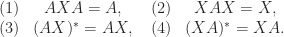
From the Moore–Penrose conditions or (1) it can be shown that $(A^+)^+ = A$ and $(A^*)^+ = (A^+)^*$ .

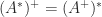
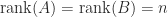
For full rank $A$ we have the concise formulas

$\notag A^+ = \begin{cases} (A^*A) ^{-1}A^*, & \textrm{if}~\mathrm{rank}(A) = n \le m, \\ A^*(AA^*)^{-1}, & \textrm{if}~ \mathrm{rank}(A) = m \le n. \end{cases} \qquad (2)$

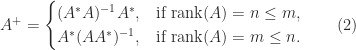
Consequently,

$\notag A^+A = I_n ~~\mathrm{if}~ \mathrm{rank}(A) = n, \qquad AA^+ = I_m ~~\mathrm{if}~ \mathrm{rank}(A) = m.$

Some special cases are worth noting.

The pseudoinverse of a zero $m\times n$ matrix is the zero $n\times m$ matrix.
The pseudoinverse of a nonzero vector $x\in\mathbb{C}^n$ is $x^*/(x^*x)$ .
For $x,y\in\mathbb{C}^n$ , $(xy^*)^+ = (y^*)^+ x^+$ and if $x$ and $y$ are nonzero then $(xy^*)^+ = yx^*/ (x^*x\cdot y^*y)$ .
The pseudoinverse of a Jordan block with eigenvalue $0$ is the transpose:

$\notag \begin{bmatrix} 0 & 1 & 0 \\ 0 & 0 & 1 \\ 0 & 0 & 0 \\ \end{bmatrix}^+ = \begin{bmatrix} 0 & 0 & 0 \\ 1 & 0 & 0 \\ 0 & 1 & 0 \end{bmatrix}.$

The pseudoinverse differs from the usual inverse in various respects. For example, the pseudoinverse of a triangular matrix is not necessarily triangular (here we are using MATLAB with the Symbolic Math Toolbox):

>> A = sym([1 1 1; 0 0 1; 0 0 1]), X = pinv(A)
A =
[1, 1, 1]
[0, 0, 1]
[0, 0, 1]
X =
[1/2, -1/4, -1/4]
[1/2, -1/4, -1/4]
[  0,  1/2,  1/2]

Furthermore, it is not generally true that $(AB)^+ = B^+A^+$ for $A\in\mathbb{C}^{m\times n}$ and $B\in\mathbb{C}^{n\times p}$ . A sufficient condition for this equality to hold is that $\mathrm{rank}(A) = \mathrm{rank}(B) = n$ .

It is not usually necessary to compute the pseudoinverse, but if it is required it can be obtained using (1) or (2) or from the Newton–Schulz iteration

$\notag X_{k+1} = 2X_k - X_kAX_k, \quad X_0 = \alpha A^*,$

for which $X_k \to A^+$ as $k\to\infty$ if $0 < \alpha < 2/\|A\|_2^2$ . The convergence is at an asymptotically quadratic rate. However, about $2\log_2\kappa_2(A)$ iterations are required to reach the asymptotic phase, where $\kappa_2(A) = \|A\|_2 \|A^+\|_2$ , so the iteration is slow to converge when $A$ is ill conditioned.

Notes and References

The pseudoinverse was first introduced by Eliakim Moore in 1920 and was independently discovered by Roger Penrose in 1955. For more on the pseudoinverse see, for example, Ben-Israel and Greville (2003) or Campbell and Meyer (2009). For analysis of the Newton–Schulz iteration see Pan and Schreiber (1991).

Adi Ben-Israel and Thomas N. E. Greville, Generalized Inverses: Theory and Applications, second edition, Springer-Verlag, New York, 2003
Stephen Campbell and Carl Meyer, Generalized Inverses of Linear Transformations, Society for Industrial and Applied Mathematics, Philadelphia, PA, USA, 2009. published (Originally published by Pitman in 1979.)
Victor Pan and Robert Schreiber, An Improved Newton Iteration for the Generalized Inverse of a Matrix, with Applications, SIAM J. Sci. Statist. Comput. 12 (5), 1109–1130, 1991.