 James Wilkinson’s 1963 book Rounding Errors in Algebraic Processes has been hugely influential. It came at a time when the effects of rounding errors on numerical computations in finite precision arithmetic had just starting to be understood, largely due to Wilkinson’s pioneering work over the previous two decades. The book gives a uniform treatment of error analysis of computations with polynomials and matrices and it is notable for making use of backward errors and condition numbers and thereby distinguishing problem sensitivity from the stability properties of any particular algorithm.
The book was originally published by Her Majesty’s Stationery Office in the UK and Prentice-Hall in the USA. It was reprinted by Dover in 1994 but has been out of print for some time. SIAM has now reprinted the book in its Classics in Applied Mathematics series. It is available from the SIAM Bookstore and, for those with access to it, the SIAM Institutional Book Collection.
I was asked to write a foreword to the book, which I include below. The photo shows Wilkinson lecturing at Argonne National Laboratory. For more about Wilkinson see the James Hardy Wilkinson web page.

Foreword
Rounding Errors in Algebraic Processes was the first book to give detailed analyses of the effects of rounding errors on a variety of key computations involving polynomials and matrices.
The book builds on James Wilkinson’s 20 years of experience in using the ACE and DEUCE computers at the National Physical Laboratory in Teddington, just outside London. The original design for the ACE was prepared by Alan Turing in 1945, and after Turing left for Cambridge Wilkinson led the group that continued to design and build the machine and its software. The ACE made its first computations in 1950. A Cambridge educated mathematician, Wilkinson was perfectly placed to develop and analyze numerical algorithms on the ACE and the DEUCE (the commercial version of the ACE). The intimate access he had to the computers (which included the ability to observe intermediate computed quantities on lights on the console) helped Wilkinson to develop a deep understanding of the numerical methods he was using and their behavior in finite precision arithmetic.
The principal contribution of the book is the analysis of the effects of rounding errors on algorithms, using backward error analysis (then in its infancy) or forward error analysis as appropriate. The book laid the foundations for the error analysis of algebraic processes on digital computers.
Three types of computer arithmetic are analyzed: floating-point arithmetic, fixed-point arithmetic (in which numbers are represented as a number on a fixed interval such as
with a fixed scale factor), and block floating-point arithmetic, which is a hybrid of floating-point arithmetic and fixed-point arithmetic. Although floating-point arithmetic dominates today’s computational landscape, fixed-point arithmetic is widely used in digital signal processing and block floating-point arithmetic is enjoying renewed interest in machine learning.
A notable feature of the book is its careful consideration of problem sensitivity, as measured by condition numbers, and this approach inspired future generations of numerical analysis textbooks.
Wilkinson recognized that the worst-case error bounds he derived are pessimistic and he noted that more realistic bounds are obtained by taking the square roots of the dimension-dependent terms (see pages 26, 52, 102, 151). In recent years, rigorous results have been derived that support Wilkinson’s intuition: they show that bounds with the square roots of the constants hold with high probability under certain probabilistic assumptions on the rounding errors.
It is entirely fitting that Rounding Errors in Algebraic Processes is reprinted in the SIAM Classics series. The book is a true classic, it continues to be well-cited, and it will remain a valuable reference for years to come.
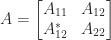
 matrix
 block
block  the Schur complement is
  . It is denoted by
  . The block with respect to which the Schur complement is taken need not be the
  is nonsingular, the Schur complement of
  is
is  .
.![\alpha = [i_1,i_2,\dots,i_k]](https://s0.wp.com/latex.php?latex=%5Calpha+%3D+%5Bi_1%2Ci_2%2C%5Cdots%2Ci_k%5D&bg=ffffff&fg=222222&s=0&c=20201002) , where
, where  , the Schur complement of
  in
in  , where
  is the complement of
  (the vector of indices not in
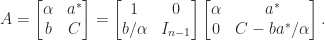
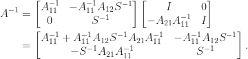
 stages of Gaussian elimination we have computed the following factorization, in which the
  :
: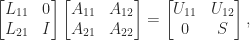
 and
and  blocks in this equation gives
 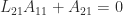 and
and 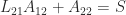 . Hence
  , which is the Schur complement of
  below the diagonal, succeeds as long as the
  ) element of
  -matrices,
 matrix. If
 is the
  .
. .
.

 , and since congruences preserve inertia (the number of positive, zero, and negative eigenvalues),
  , where “+” denotes the Moore-Penrose pseudo-inverse. The generalized Schur complement is useful in the context of Hermitian positive semidefinite matrices, as the following result shows.
 and
and 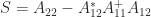 are both positive semidefinite.
