
The MATLAB function sqrtm, for computing a square root of a matrix, first appeared in the 1980s. It was improved in MATLAB 5.3 (1999) and again in MATLAB 2015b. In this post I will explain how the recent changes have brought significant speed improvements.
Recall that every 


In practice, it is usually the principal square root that is wanted, which is the one whose eigenvalues lie in the right-half plane. This square root is unique if
The original sqrtm transformed
The importance of sqrtm has grown over the years because logm (for the matrix logarithm) depends on it, as do codes for other matrix functions, for computing arbitrary powers of a matrix and inverse trigonometric and inverse hyperbolic functions.
For a triangular matrix 


The new sqrtm introduced in MATLAB 2015b contains a new implementation of the Björck–Hammarling recurrence that, while still in M-code, is much faster. Here is a comparison of the underlying function sqrtm_tri (contained in toolbox/matlab/matfun/private/sqrtm_tri.m) with the relevant piece of code extracted from the old sqrtm. Shown are execution times in seconds for random triangular matrices an a quad-core Intel Core i7 processor.
| n | sqrtm_tri |
old sqrtm |
|---|---|---|
| 10 | 0.0024 | 0.0008 |
| 100 | 0.0017 | 0.014 |
| 1000 | 0.45 | 3.12 |
For 


How does sqrtm_tri work? It uses a recursive partitioning technique. It writes

and notes that
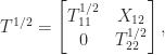
where 


edit private/sqrtm_tri at the MATLAB prompt. For more on this recursive scheme for computing square roots of triangular matrices see Blocked Schur Algorithms for Computing the Matrix Square Root (2013) by Deadman, Higham and Ralha.
The sqrtm in MATLAB 2015b includes two further refinements.
- For real matrices it uses the real Schur form, which means that all computations are carried out in real arithmetic, giving a speed advantage and ensuring that the result will not be contaminated by imaginary parts at the roundoff level.
- It estimates the 1-norm condition number of the matrix square root instead of the 2-norm condition number, so exploits the normest1 function.
Finally, I note that the product of two triangular matrices is also not a level-3 BLAS routine, yet again it is needed in matrix function codes. A proposal for it to be included in the Intel Math Kernel Library was made recently by Peter Kandolf, and I strongly support the proposal.

 , instead of bounding the
  th term
  by
by  , a potentially smaller bound is used.
  and are not willing to compute
  but are willing to compute lower powers of
  , so
, so  ,
,  ,
,  , and
, and  . But it is easy to see that
  and
and  , so we can discard two of the bounds, ending up with
 for values of
  up to some small, fixed value. The gains can be significant. Consider the matrix
 , but
, but 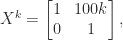
 , which is a significant improvement.
 is the spectral radius (the largest modulus of any eigenvalue). The upper bound corresponds to the usual analysis. The lower bound is something that we cannot use to bound the norm of the power series. The middle term is what we are using, and as
  the middle term converges to the lower bound, which can be arbitrarily smaller than the upper bound.

 denotes a particular branch of the logarithm—possibly different in each case. In other words, the equation is true for the multivalued function that includes all branches.
 lies in the interval
 ![(-\pi,\pi]](https://s0.wp.com/latex.php?latex=%28-%5Cpi%2C%5Cpi%5D&bg=ffffff&fg=222222&s=0&c=20201002) (or possibly some other specific branch). Now the equation is not always true. A correction term that makes the equation valid can be expressed in terms of the unwinding number introduced by Corless, Hare, and Jeffrey in 1996, which is discussed in my earlier post
(or possibly some other specific branch). Now the equation is not always true. A correction term that makes the equation valid can be expressed in terms of the unwinding number introduced by Corless, Hare, and Jeffrey in 1996, which is discussed in my earlier post  is not equivalent to
  for complex
  ). This is a good way to proceed, but working out the ranges of the principal functions from these definitions is not trivial.
 equal to


 . We are now seeing growing use of mixed precision, in which different floating point precisions are combined in order to deliver a result of the required accuracy at minimal cost.
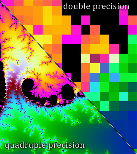
 , is good enough for training and running neural networks. Here are some of the ways in which extra precision is currently being used.
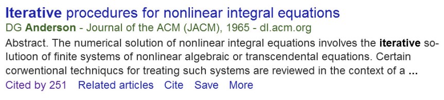 I learned about Anderson acceleration in the minisymposium

 and
and  to write
  . The ISS algorithm for the matrix case uses the same idea, with the square roots being matrix square roots, but approximates
  at a matrix argument using Padé approximants, evaluated using a partial fraction expansion. The Fréchet derivative of the logarithm can be obtained by Fréchet differentiating the formulas used in the ISS algorithm. For details see
  of
of  . Its many applications include the solution of delay differential equations. Rob Corless and his colleagues produced a
  function does not yield all solutions to
  , just as the primary logarithm does not yield all solutions to
  . I am involved in some further work on the matrix Lambert W function and hope to have more to report in due course.
 real or complex matrix. Consider the principal logarithm—the one for which
  for
for  (an important special case being
  for an integer
  for all
  for all
  whenever
  commute.
 is always true.
 is false.
 in the above expressions stands for the families of all possible logarithms and powers then the identities are all true. But from a computational viewpoint we are usually concerned with a particular branch of each function, the principal branch, so equality cannot be taken for granted.
 , and it arises from the scalar unwinding number introduced by Corless, Hare and Jeffrey in 1996
 , so the relation in the first quiz question is clearly valid when
  , which is the case when the eigenvalues of
 and the matrix
  has eigenvalues with imaginary parts in
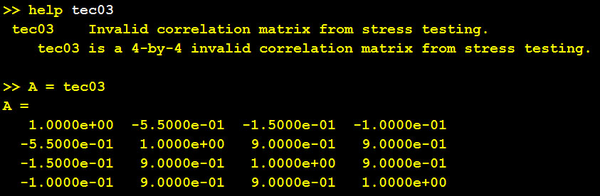
  ? The following incomplete MATLAB code implements the Schur algorithm developed in the paper. The