What Is the Sherman–Morrison–Woodbury Formula?

When a nonsingular $n\times n$ matrix $A$ is perturbed by a matrix of rank $k$ , the inverse also undergoes a rank- $k$ perturbation. More precisely, if $E$ has rank $k$ and $B = A+E$ is nonsingular then the identity $A^{-1} - B^{-1} = A^{-1} (B-A) B^{-1}$ shows that

$\notag \mathrm{rank}(A^{-1} - B^{-1}) = \mathrm{rank}(A^{-1} E B^{-1}) = \mathrm{rank}(E) = k.$

The Sherman–Morrison–Woodbury formula provides an explicit formula for the inverse of the perturbed matrix $B$ .

Sherman–Morrison Formula

We will begin with the simpler case of a rank- $1$ perturbation: $B = A + uv^*$ , where $u$ and $v$ are $n$ -vectors, and we consider first the case where $A = I$ . We might expect that $(I + uv^*)^{-1} = I + \theta uv^*$ for some $\theta$ (consider a binomial expansion of the inverse). Multiplying out, we obtain

$\notag (I + uv^*) (I + \theta uv^*) = I + (1 + \theta + \theta v^*u) uv^*,$

so the product equals the identity matrix when $\theta = -1/(1 + v^*u)$ . The condition that $I + uv*$ be nonsingular is $v^*u \ne -1$ (as can also be seen from $\det(I + uv^*) = 1 + v^*u$ , derived in What Is a Block Matrix?). So

$\notag (I + uv^*)^{-1} = I - \displaystyle\frac{1}{1 + v^*u} uv^*.$

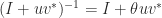
For the general case write $B = A + uv^* = A(I + A^{-1}u v^*)$ . Inverting this equation and applying the previous result gives

$\notag (A + uv^*)^{-1} = A^{-1} - \displaystyle\frac{A^{-1} uv^* A^{-1}}{1 + v^* A^{-1} u},$

subject to the nonsingularity condition $v^*A^{-1}x \ne -1$ . This is known as the Sherman–Morrison formula. It explicitly identifies the rank- $1$ change to the inverse.

As an example, if we take $u = te_i$ and $v = e_j$ (where $e_k$ is the $k$ th column of the identity matrix) then, writing $A^{-1} = (\alpha_{ij})$ , we have

$\notag \bigl(A + te_ie_j^*\bigr)^{-1} = A^{-1} - \displaystyle\frac{tA^{-1}e_i e_j^* A^{-1}}{1 + t \alpha_{ji}}.$

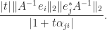
The Frobenius norm of the change to $A^{-1}$ is

$\notag \displaystyle\frac{ |t|\, \| A^{-1}e_i\|_2 \| e_j^*A^{-1}\|_2 } {|1 + t \alpha_{ji}|}.$

If $t$ is sufficiently small then this quantity is approximately maximized for $i$ and $j$ such that the product of the norms of $i$ th column and $j$ th row of $A^{-1}$ is maximized. For an upper triangular matrix $i = n$ and $j = 1$ are likely to give the maximum, which means that the inverse of an upper triangular matrix is likely to be most sensitive to perturbations in the $(n,1)$ element of the matrix. To illustrate, we consider the matrix

$\notag T = \left[\begin{array}{rrrr} 1 & -1 & -2 & -3\\ 0 & 1 & -4 & -5\\ 0 & 0 & 1 & -6\\ 0 & 0 & 0 & 1 \end{array}\right]$

The $(i,j)$ element of the following matrix is $\| T^{-1} - (T + 10^{-3}e_ie_j^*)^{-1} \|_F$ :

$\notag \left[\begin{array}{cccc} 0.044 & 0.029 & 0.006 & 0.001 \\ 0.063 & 0.041 & 0.009 & 0.001 \\ 0.322 & 0.212 & 0.044 & 0.007 \\ 2.258 & 1.510 & 0.321 & 0.053 \\ \end{array}\right]$

As our analysis suggests, the $(4,1)$ entry is the most sensitive to perturbation.

Sherman–Morrison–Woodbury Formula

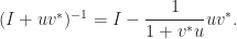
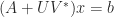
Now consider a perturbation $UV^*$ , where $U$ and $V$ are $n\times k$ . This perturbation has rank at most $k$ , and its rank is $k$ if $U$ and $V$ are both of rank $k$ . If $I + V^* A^{-1} U$ is nonsingular then $A + UV^*$ is nonsingular and

$\notag (A + UV^*)^{-1} = A^{-1} - A^{-1} U (I + V^* A^{-1} U)^{-1} V^* A^{-1},$

which is the Sherman–Morrison–Woodbury formula. The significance of this formula is that $I + V^* A^{-1} U$ is $k\times k$ , so if $k\ll n$ and $A^{-1}$ is known then it is much cheaper to evaluate the right-hand side than to invert $A + UV^*$ directly. In practice, of course, we rarely invert matrices, but rather exploit factorizations of them. If we have an LU factorization of $A$ then we can use it in conjunction with the Sherman–Morrison–Woodbury formula to solve $(A + UV^*)x = b$ in $O(n^2 + k^3)$ flops, as opposed to the $O(n^3)$ flops required to factorize $A + UV^*$ from scratch.

The Sherman–Morrison–Woodbury formula is straightforward to verify, by showing that the product of the two sides is the identity matrix. How can the formula be derived in the first place? Consider any two matrices $F$ and $G$ such that $FG$ and $GF$ are both defined. The associative law for matrix multiplication gives $F(GF) = (FG)F$ , or $(I + FG)F = F (I + GF)$ , which can be written as $F(I+GF)^{-1} = (I+FG)^{-1}F$ . Postmultiplying by $G$ gives

$\notag F(I+GF)^{-1}G = (I+FG)^{-1}FG = (I+FG)^{-1}(I + FG - I) = I - (I+FG)^{-1}.$

Setting $F = U$ and $G = V^*$ gives the special case of the Sherman–Morrison–Woodbury formula with $A = I$ , and the general formula follows from $A + UV^* = A(I + A^{-1}U V^*)$ .

General Formula

We will give a different derivation of an even more general formula using block matrices. Consider the block matrix

$\notag X = \begin{bmatrix} A & U \\ V^* & -W^{-1} \end{bmatrix}$

where $A$ is $n\times n$ , $U$ and $V$ are $n\times k$ , and $W$ is $k\times k$ . We will obtain a formula for $(A + UWV^*)^{-1}$ by looking at $X^{-1}$ .

It is straightforward to verify that

$\notag \begin{bmatrix} A & U \\ V^* & -W^{-1} \end{bmatrix} = \begin{bmatrix} I & 0 \\ V^*A^{-1} & I \end{bmatrix} \begin{bmatrix} A & 0 \\ 0 & -(W^{-1} + V^*A^{-1}U) \end{bmatrix} \begin{bmatrix} I & A^{-1}U \\ 0 & I \end{bmatrix}.$

Hence

$\notag \begin{aligned} \begin{bmatrix} A & U \\ V^* & -W^{-1} \end{bmatrix}^{-1} &= \begin{bmatrix} I & -A^{-1}U \\ 0 & I \end{bmatrix}. \begin{bmatrix} A^{-1} & 0 \\ 0 & -(W^{-1} + V^*A^{-1}U)^{-1} \end{bmatrix} \begin{bmatrix} I & 0 \\ -V^*A^{-1} & I \end{bmatrix}\\[\smallskipamount] &= \begin{bmatrix} A^{-1} - A^{-1}U(W^{-1} + V^*A^{-1}U)^{-1}V^*A^{-1} & A^{-1}U(W^{-1} + V^*A^{-1U})^{-1} \\ (W^{-1} + V^*A^{-1}U)^{-1} V^*A^{-1} & -(W^{-1} + V^*A^{-1}U)^{-1} \end{bmatrix}. \end{aligned}$

In the $(1,1)$ block we see the right-hand side of a Sherman–Morrison–Woodbury-like formula, but it is not immediately clear how this relates to $(A + UWV^*)^{-1}$ . Let $P = \bigl[\begin{smallmatrix} 0 & I \\ I & 0 \end{smallmatrix} \bigr]$ , and note that $P^{-1} = P$ . Then

$\notag PXP = \begin{bmatrix} -W^{-1} & V^* \\ U & A \end{bmatrix}$

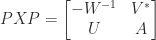
and applying the above formula (appropriately renaming the blocks) gives, with $\times$ denoting a block whose value does not matter,

$\notag PX^{-1}P = (PXP)^{-1} = \begin{bmatrix} \times & \times \\ \times & (A + UWV^*)^{-1} \end{bmatrix}.$

Hence $(X^{-1})_{11} = (A + UWV^*)^{-1}$ . Equating our two formulas for $(X^{-1})_{11}$ gives

$\notag \qquad\qquad\qquad (A + UWV^*)^{-1} = A^{-1} - A^{-1}U (W^{-1} + V^*A^{-1}U)^{-1} V^*A^{-1}, \qquad\qquad\qquad(*)$

provided that $W^{-1} + V^*A^{-1}U$ is nonsingular.

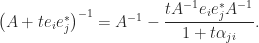
To see one reason why this formula is useful, suppose that the matrix $A$ and its perturbation are symmetric and we wish to preserve symmetry in our formulas. The Sherman–Morrison–Woodbury requires us to write the perturbation as $UU^*$ , so the perturbation must be positive semidefinite. In $(*)$ , however, we can write an arbitrary symmetric perturbation as $UWU^*$ , with $W$ symmetric but possibly indefinite, and obtain a symmetric formula.

The matrix 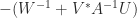$-(W^{-1} + V^*A^{-1}U)$ is the Schur complement of $A$ in $X$ . Consequently the inversion formula $(*)$ is intimately connected with the theory of Schur complements. By manipulating the block matrices in different ways it is possible to derive variations of $(*)$ . We mention just the simple rewriting

$\notag (A + UWV^*)^{-1} = A^{-1} - A^{-1}U W(I + V^*A^{-1}UW)^{-1} V^*A^{-1},$

which is valid if $W$ is singular, as long as $I + WV^*A^{-1}U$ is nonsingular. Note that the formula is not symmetric when $V = U$ and $W = W^*$ . This variant can also be obtained by replacing $U$ by $UW$ in the Sherman–Morrison–Woodbury formula.

Historical Note

Formulas for the change in a matrix inverse under low rank perturbations have a long history. They have been rediscovered on multiple occasions, sometimes appearing without comment within other formulas. Equation $(*)$ is given by Duncan (1944), which is the earliest appearance in print that I am aware of. For discussions of the history of these formulas see Henderson and Searle (1981) or Puntanen and Styan (2005).

References

This is a minimal set of references, which contain further useful references within.

W. J. Duncan, LXXVIII. Some Devices for the Solution of Large Sets of Simultaneous Linear Equations, The London, Edinburgh, and Dublin Philosophical Magazine and Journal of Science 35, 660–670, 1944.
H. V. Henderson and S. R. Searle, On Deriving the Inverse of a Sum of Matrices, SIAM Rev. 23(1), 53–60, 1981.
Simo Puntanen and George Styan, Historical Introduction: Issai Schur and the Early Development of the Schur Complement, pages 1-16 in Fuzhen Zhang, ed., The Schur Complement and Its Applications, Springer-Verlag, New York, 2005.

4 thoughts on “What Is the Sherman–Morrison–Woodbury Formula?”

Carlos says:

September 29, 2020 at 11:17 am

Hi!
Right before the section ‘General Formula’, it seems that the expression is missing a parenthesis: A + UV* = A(1 – A)^-1 UV*
Thanks for this nice post!
Cheers.

1. Nick Higham says:
  
  September 29, 2020 at 11:27 am
  
  Thanks – corrected.
  
  1. Carlos Frederico says:
    
    September 29, 2020 at 11:41 am
    
    I clearly mistaken the factorization of A. Thanks for the correction!
    
Timo Euler says:

October 7, 2020 at 10:52 am

While using Sherman-Morrison-Woodbury for deriving results for exponential and other functions of perturbed matrices for some time, I finally stumbled across your Theorem 1.35 in “N. J. Higham, Functions of Matrices: Theory and Computation, SIAM, 2008.” This theorem is simply: beautiful! I love it! It is a wonderful generalization of Sherman-Morrison-Woodbury and renders my former tedious calculations short and easy ones while lifting the caveats on corner cases. Easy to code, too. Thanks!
So, if you are in need for calculating functions on low-rank perturbed matrices: take a look at Theorem 1.35 🙂

What Is the Sherman–Morrison–Woodbury Formula?

Sherman–Morrison Formula

Sherman–Morrison–Woodbury Formula

General Formula

Historical Note

References

Related Blog Posts

4 thoughts on “What Is the Sherman–Morrison–Woodbury Formula?”

Leave a Reply to Carlos Cancel reply

Sherman–Morrison Formula

Sherman–Morrison–Woodbury Formula

General Formula

Historical Note

References

Related Blog Posts

Share this:

Related

4 thoughts on “What Is the Sherman–Morrison–Woodbury Formula?”

Leave a Reply to Carlos Cancel reply