I didn’t have time earlier this year to write about the first MATLAB release of 2019, so in this post I will discuss R2019a and R2019b together. As usual in this series, I concentrate on the features most relevant to my work.
Modified Akima Cubic Hermite Interpolation (R2019b)

A new function makima computes a piecewise cubic interpolant with continuous first-order derivatives. It produces fewer undulations than the existing spline function, with less flattening than pchip. This form of interpolant has been an option in interp1, interp2, interp3, interpn, and griddedInterpolant since R2017b and is now also a standalone function. For more details see Cleve Moler’s blog post about makima, from which the code used to generate the image above is taken.
Linear Assignment Problem and Equilibration (R2019a)
The matchpairs function solves the linear assignment problem, which requires each row of a matrix to be assigned to a column in such a way that the total cost of the assignments (given by the “sum of assigned elements” of the matrix) is minimized (or maximized). This problem can also be described as finding a minimum-weight matching in a weighted bipartite graph. The problem arises in sparse matrix computations.
The equilibrate function take as input a matrix A (dense or sparse) and returns a permutation matrix P and nonsingular diagonal matrices R and C such that R*P*A*C has diagonal entries of magnitude 1 and off-diagonal entries of magnitude at most 1. The outputs P, R, and C are sparse. This matrix equilibration can improve conditioning and can be a useful preprocessing step both in computing incomplete LU preconditioners and in iterative solvers. See, for example, the recent paper Max-Balanced Hungarian Scalings by Hook, Pestana, Tisseur, and Hogg.
The scaling produced by equilibrate is known as Hungarian scaling, and its computation involves solving a linear assignment problem.
Function Argument Validation (R2019b)
A powerful new feature allows a function to check that its input arguments have the desired class, size, and other aspects. Previously, this could be done by calling the function validateattributes with each argument in turn or by using the inputParser object (see Loren Shure’s comparison of the different approaches).
The new feature provides a more structured way of achieving the same effect. It also allows default values for arguments to be specified. Function argument validation contains many aspects and has a long help page. We just illustrate it with a simple example that should be self-explanatory.
function fav_example(a,b,f,t)
  arguments
    a (1,1) double               % Double scalar.
    b {mustBeNumeric,mustBeReal} % Numeric type and real.
    f double {mustBeMember(f,[-1,0,1])} = 0 % -1, 0 (default), or 1.
    t string = "-"               % String, with default value.
  end
  % Body of function.
end
The functions mustBeNumeric and mustBeMember are just two of a long list of validation functions. Here is an example call:
>> a = 0; b = 2; f = 11; fav_example(a,b,f)
Error using fav_example
Invalid input argument at position 3. Value must be a member of ...
this set:
    -1
    0
    1
One caveat is that a specification within the arguments block
v (1,:) double
allows not just 1-by-n vectors (for any n) but also n-by-1 vectors, because of the convention that in many situations MATLAB does not distinguish between row and column vectors.
For more extensive examples, see New with R2019b – Function Argument Validation and Spider Plots and More Argument Validation by Jiro Doke at MathWorks Blogs.
Dot Indexing (R2019b)
One can now dot index the result of a function call. For example, consider
>> optimset('Display','iter').Display
ans =
    'iter'
The output of the dot call can even be indexed:
>> optimset('OutputFcn',{@outfun1,@outfun2}).OutputFcn{2}
ans =
  function_handle with value:
    @outfun2
Of course, these are contrived examples, but in real codes such indexing can be useful. This syntax was not allowed in R2019a and earlier.
Hexadecimal and Binary Values (R2019b)
One can now specify hexadecimal and binary values using the prefixes 0x or 0X for hexadecimal (with upper or lower case for A to F) and 0b or 0B for binary. By default the results have integer type.
>> 0xA
ans =
  uint8
   10
>> 0b101
ans =
  uint8
   5
Changes to Function Precedence Order (R2019b)
The Release Notes say “Starting in R2019b, MATLAB changes the rules for name resolution, impacting the precedence order of variables, nested functions, local functions, and external functions. The new rules simplify and standardize name resolution”. A number of examples are given where the meaning of code is different in R2019b, and they could cause an error to be generated for codes that ran without error in earlier versions. As far as I can see, though, these changes are not likely to affect well-written MATLAB code.
Program File Size (R2019b)
Program files larger than “approximately 128 MB” will no longer open or run. This is an interesting change because I cannot imagine writing an M-file of that size. Good programming practice dictates splitting a code into separate functions and not including all of them in one program file. Presumably, some MATLAB users have produced such long files—perhaps automatically generated.
For a modern introduction and reference to MATLAB, see MATLAB Guide (third edition, 2017)


 . Thus
 s and
s and  s:
s: factor in the LU factorization with partial pivoting of
  , and these entries are not all integers. Standard rounding error analysis shows that the relative error from forming that product is bounded by
  , with
  , where
 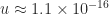 is the unit roundoff, and this is comfortably larger than the actual relative error (which also includes the errors in computing
  . Therefore the computed determinant is well within the bounds of roundoff, and if the exact result had not been an integer the incorrect last decimal digit would hardly merit discussion.
 ) is standard notation for a perturbation of the matrix
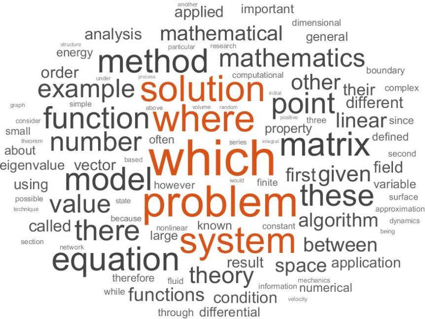
 Wordle removes certain stop words (common but unimportant words) that

 can be represented by a pair of double precision numbers
  , where
  and
and  and
and  represent the leading and trailing significant digits of
  can be written
  , which involves four double precision multiplications and three double precision additions. We can therefore expect quadruple precision multiplication to be at least seven times slower than double precision multiplication. Almost all available implementations of quadruple precision arithmetic are in software (an exception is provided by the


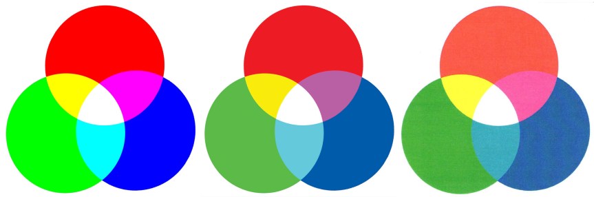 The differences between the RGB version and the other two versions may be shocking! Fortunately, when the CMYK version is viewed on a printed page in isolation from the RGB version (necessarily displayed on a monitor) it does not look so bad. [Of course, if you are reading a printed version of this post then the first two images will look essentially the same.]
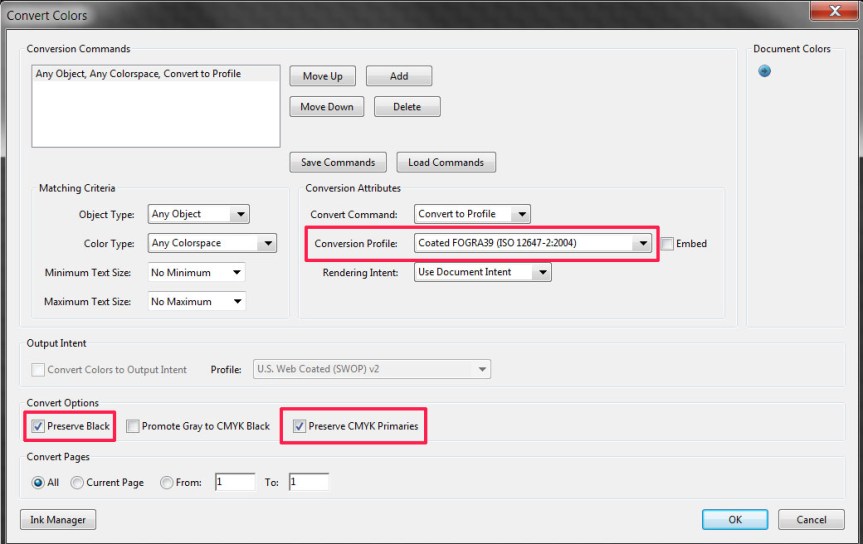 There are a couple of things to note. First, Adobe Acrobat does not remember the settings in the dialog box, so they need to be re-entered every time. Second, since “Embed profile” is not selected with the settings shown, there is no way to tell which profile has been used once the conversion has been done.
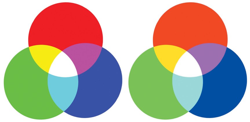 On the left is the result of converting the original RGB image to “U.S. Web Coated (SWOP) v2” and on the right is the result of converting to “Photoshop 5 default CMYK” (and converting back to RGB in both cases, the latter conversion producing no visual difference in Photoshop). There is a significant difference between the two conversions in every color except white! In principle, both conversions will produce the same result when printed with the target ink and paper, but if you choose the profile without knowing the target you have little idea what the printed result will be.