This post is an edited and updated version of an article that I published in 2006 in the IMANA Newsletter (“Newsletter of the Numerical Analysis Group of the Institute of Mathematics and its Applications”). Very few issues of the Newsletter appear to be electronically available, so I thought it worthwhile to reproduce the article here.
The University of Manchester Numerical Analysis (NA) Report series began in 1974. The two key movers in setting up the series were Ian Gladwell, a member of the Department of Mathematics at the University of Manchester (now retired from the Department of Mathematics at Southern Methodist University, Dallas), and Charlie Van Loan, an SERC-funded postdoctoral visitor to the department in 1974–1975 (and subsequently a professor in the Department of Computer Science at Cornell University). The first report was
Charles F. Van Loan, Least Squares Problems with Emphasis Upon Singular Value Techniques, Numerical Analysis Report No. 1, September 1974.
and Charlie wrote four of the first 10 reports. Particularly notable is
Charles F. Van Loan. A study of the matrix exponential. Numerical Analysis Report No. 10, August 1975.
This was an early version of the classic, highly-cited article “Nineteen Dubious Ways to Compute the Exponential of a Matrix” written with Cleve Moler and subsequently published in SIAM Review in 1978, with an updated reprint in SIAM Review in 2003. The report has been reissued as MIMS EPrint 2206.397. Ian’s early contributions include the often-cited
J. L. Siemieniuch and I. Gladwell On time discretization for linear time-dependent partial differential equations. Numerical Analysis Report No. 5, September 1974.
One of the main aims of the series was to provide a vehicle for pre-publication of a preliminary version of a piece of work, prior it to being submitted to a journal. Right from the start this aim was achieved, with at least 15 of the first 20 reports known to have appeared in refereed journals. Nevertheless, a number of important early reports, such as Number 5 mentioned above, were not submitted but surely would have been in today’s academic climate.
The contents of the series naturally reflect the interests of the numerical analysts at the University of Manchester and UMIST over the years. The first 125 reports (taking us up to October 1986) include contributions on stiff differential equations (George Hall, Jack Williams), complex approximation (Jack Williams), Volterra integral equations (Christopher Baker), polynomial zero-finding (Len Freeman), methods for second order ordinary differential equations (Ian Gladwell, Ruth Thomas), multigrid (Joan Walsh), numerical linear algebra (Nick Higham), and numerical analysis of partial differential equations (Ian Gladwell, David Silvester, Ron Thatcher, Joan Walsh).
As well as containing preprints of research papers, the series includes all thirteen Annual Reports of the Manchester Centre for Computational Mathematics and the proceedings of two 1982 meetings:
Ian Gladwell (ed.), Proceedings of a One-Day Colloquium On Numerical Linear Algebra and Its Applications. Numerical Analysis Report No. 78, July 1982.
George Hall and Jack Williams (eds), Proceedings of a One-Day Colloquium on the Numerical Solution of Ordinary Differential Equations. Numerical Analysis Report No. 84, December 1982.
The reports illustrate the changes in typesetting mathematics since the 1970s. Early reports were typewritten, sometimes with equations written in by hand. In the 1980s many of the reports were wordprocessed using Vuwriter—a technical wordprocessor produced by Vuman Ltd., a spin-off company of the University of Manchester, targeted at the Apricot microcomputer. I wordprocessed several reports on a Commodore 64 microcomputer using an Epson printer, with Greek letters and mathematical characters produced in the printer’s graphics mode (see this earlier post for more details).
The first TeXed reports were around 1986/1987 and by the early 1990s most reports were produced in  , as they are today.
The printed reports retained their distinctive green card cover to the end, but a major change came in May 1993 when they were first made available over the internet—originally by anonymous ftp from vtx.ma.man.ac.uk and then from the Manchester Centre for Computational Mathematics (MCCM) web site set up in 1994. The web page from which the reports are available, now located here, was automatically created from a BibTeX bib file, the latter being maintained by hand, as was the repository of PDF and PS files.
In 2005, the NA Report series was folded into the new MIMS EPrints archive (http://eprints.ma.man.ac.uk/) which hosts research outputs of members of the School of Mathematics and associated researchers. EPrints entries are assigned an AMS subject classification and can be searched by those numbers. Reports that would have appeared in the old NA Report series can now generally be found under the classification 65 Numerical Analysis.
On a recent visit to the University of Manchester library I was pleased to find that many of the NA reports up to 2001 are still available in hard copy on the shelves. (A search of the catalogue for “numerical analysis report” reveals the details.)
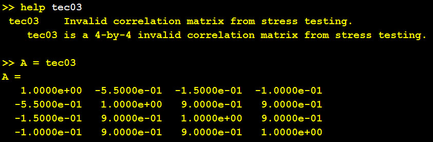

 . A 1989 MATLAB manual says


 , instead of bounding the
  th term
  by
by  , a potentially smaller bound is used.
  and are not willing to compute
  but are willing to compute lower powers of
  . We have
  , so
, so  ,
,  ,
,  , and
, and  . But it is easy to see that
 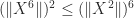 and
and 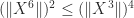 , so we can discard two of the bounds, ending up with
 for values of
  up to some small, fixed value. The gains can be significant. Consider the matrix
 , but
, but 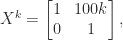
 , which is a significant improvement.
 is the spectral radius (the largest modulus of any eigenvalue). The upper bound corresponds to the usual analysis. The lower bound is something that we cannot use to bound the norm of the power series. The middle term is what we are using, and as
  the middle term converges to the lower bound, which can be arbitrarily smaller than the upper bound.


 denotes a particular branch of the logarithm—possibly different in each case. In other words, the equation is true for the multivalued function that includes all branches.
 lies in the interval
 ![(-\pi,\pi]](https://s0.wp.com/latex.php?latex=%28-%5Cpi%2C%5Cpi%5D&bg=ffffff&fg=222222&s=0&c=20201002) (or possibly some other specific branch). Now the equation is not always true. A correction term that makes the equation valid can be expressed in terms of the unwinding number introduced by Corless, Hare, and Jeffrey in 1996, which is discussed in my earlier post
(or possibly some other specific branch). Now the equation is not always true. A correction term that makes the equation valid can be expressed in terms of the unwinding number introduced by Corless, Hare, and Jeffrey in 1996, which is discussed in my earlier post  is not equivalent to
  for complex
  ). This is a good way to proceed, but working out the ranges of the principal functions from these definitions is not trivial.
 equal to
  ?”—see our recent EPrint


 should be in roman font. However, standard
  ) instead of
  ). The best way to define macros for additional functions is via
  ; and combined with a letter to denote a variable, hence italic, as in
  (where in
  instead of
  . This certainly follows the rules above, since such polynomials have a fixed meaning, but I have never seen the upright font being used for such polynomials in practice.