What effect does a rank-1 perturbation of norm 1 to an 

Consider first a perturbation of the identity matrix: 


Another example is 


Let’s take a random orthogonal matrix and perturb it with a random rank-1 matrix of unit norm. We use the following MATLAB code.
n = 100; rng(1)
A = gallery('qmult',n); % Random Haar distrib. orthogonal matrix.
x = randn(n,1); y = randn(n,1);
x = x/norm(x); y = y/norm(y);
B = A + x*y';
svd_B = svd(B);
max_svd_B = max(svd_B), min_svd_B = min(svd_B)
The output is
max_svd_B =
1.6065e+00
min_svd_B =
6.0649e-01
We started with a matrix having singular values all equal to 1 and now have a matrix with largest singular value a little larger than 1 and smallest singular value a little smaller than 1. If we keep running this code the extremal singular values of
max_svd_B =
1.5921e+00
min_svd_B =
5.9213e-01
A rank-1 perturbation of unit norm could make
What is the explanation? First, note that a rank-1 perturbation to an orthogonal matrix 

A result of Benaych-Georges and Nadakuditi (2012) says that for large 

The result in question requires the original orthogonal matrix to be from the Haar distribution, and such matrices can be generated by A = gallery('qmult',n) or by the construction
[Q,R] = qr(randn(n));
Q = Q*diag(sign(diag(R)));
(See What Is a Random Orthogonal Matrix?.) The result also requires 

However, as the next example shows, the perturbed singular values can be close to the values that the Benaych-Georges and Nadakuditi result predicts even when the conditions of the result are violated:
n = 100; rng(1)
A = gallery('orthog',n);   % Random orthogonal matrix (not Haar).
x = rand(n,1); y = (1:n)'; % Non-random y.
x = x/norm(x); y = y/norm(y);
B = A + x*y';
svd_B = svd(B);
max_svd_B = max(svd_B), min_svd_B = min(svd_B)
max_svd_B =
1.6069e+00
min_svd_B =
6.0687e-01
The question of the conditioning of a rank-1 perturbation of an orthogonal matrix arises in the recent EPrint Random Matrices Generating Large Growth in LU Factorization with Pivoting.


 is the precision and
 ![e\in [e_{\min},e_{\max}]](https://s0.wp.com/latex.php?latex=e%5Cin+%5Be_%7B%5Cmin%7D%2Ce_%7B%5Cmax%7D%5D&bg=ffffff&fg=222222&s=0&c=20201002) is the exponent. The significand
is the exponent. The significand  is an integer satisfying
  . Numbers with
  are called normalized. Subnormal numbers, for which
  and
and  , are supported.
 .
.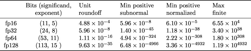 Fp32 (single precision) and fp64 (double precision) were in the 1985 standard; fp16 (half precision) and fp128 (quadruple precision) were introduced in 2008. Fp16 is defined only as a storage format, though it is widely used for computation.
 (usually written as inf in programing languages) as floating-point numbers: every arithmetic operation produces a number in the system. A NaN is generated by operations such as

 evaluates as
  when
when  .
.
 denotes the computed result. The standard also includes a fused multiply-add operation (FMA),
  . The definition requires it to be computed with just one rounding error, so that
  is the rounded version of
  , and hence satisfies
 ) and transcendental functions (
 ,
,  ,
,  ,
,  , etc.) and defines domains and special values for them, but these functions are not required.
 along with the error
  , for
, for  . These operations are useful for implementing compensated summation and other special high accuracy algorithms.
 is a finite subset of the real line comprising numbers of the form
 is the base,
  , and
, and  . The significand
  . Normalized numbers are those for which
  , and they have a unique representation. Subnormal numbers are those with
  and
and  is
is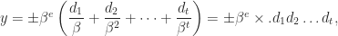
 satisfies
 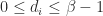 and
and  for normalized numbers.
 ,
,  , and
, and ![e \in [-1, 3]](https://s0.wp.com/latex.php?latex=e+%5Cin+%5B-1%2C+3%5D&bg=ffffff&fg=222222&s=0&c=20201002) .
.
 and
and  , which is called the machine epsilon. Note that
  .
. and the smallest normalized number, which is
  . The subnormal numbers fill this gap with numbers having the same spacing as those between
  , namely
  . The next diagram shows the complete set of nonnegative normalized and subnormal numbers in the toy system.
 . If
. If  then
then  ; otherwise,
  and
and  then
then 
 ,
,  ,
,  ,
,  , and
, and  are usually defined to return the correctly rounded exact result, so they satisfy
 , so all the numbers are equally spaced. In most scientific computations scale factors must be introduced in order to be able to represent the range of numbers occurring. Fixed-point arithmetic is mainly used on special purpose devices such as FPGAs and in embedded systems.
 to
to  , which can be described as rounding to three significant digits or two decimal places. Rounding does not change a number if it already has the requisite number of digits.
 ,
,  , or
, or  in floating-point arithmetic,
 and
and  and
and  , respectively, from
  to two significant digits, the result is
  with round to even and
  with round to odd.
 ,
,  ,
,  ,
,  ,
,  ,
,  with round to odd.
 or less and otherwise round up.
 rounds to
  . Similarly, with round towards minus infinity (or round down) we round to the next smaller number, so that
  .
. and round it up if
  . This is also known as chopping, or truncation.
 be the candidates for the result of rounding. We round up to
  with probability
  and down to
  with probability
  ; note that these probabilities sum to
  ), and round towards minus infinity (
 ). They show the number
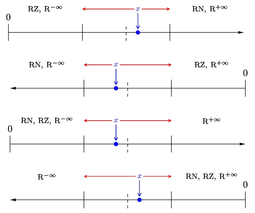
 C and
C and  F round to
  C and
C and  F instead of
  C and
C and  F.
F. package
  is orthogonal and symmetric and we can choose the nonzero vector
  is from the Haar distribution then so is
  for any orthogonal (possibly non-random)
  and
and  . A random Householder matrix is not Haar distributed.
 has nonnegative diagonal elements. This construction requires
  flops.
 be an
be an  -vector of elements from the standard normal distribution and let
  be the Householder matrix that reduces
  , where
  is the first unit vector. Then
  is Haar distributed, where
  ,
,  , and
, and  . This construction expresses
  flops. The MATLAB statement
  , where the elements of
  (where
  is symmetric positive semidefinite).
 .
. are column vectors with
  element
 is the mean of the elements in
  . If
. If 
 . The
. The  is the correlation between the variables
  .
.![[-1, 1]](https://s0.wp.com/latex.php?latex=%5B-1%2C+1%5D&bg=ffffff&fg=222222&s=0&c=20201002) .
.![[0,n]](https://s0.wp.com/latex.php?latex=%5B0%2Cn%5D&bg=ffffff&fg=222222&s=0&c=20201002) .
.
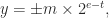
 ,
,  ,
,  . The only value of
  and
and  that makes
  with every off-diagonal element equal to
  , illustrated for
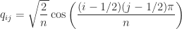
  by
by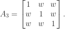
 .
. , so we solve the problem
 remain fixed. And we may want to weight some elements more than others, by using a weighted Frobenius norm. These are convex optimization problems and have a unique solution that can be computed using the alternating projections method (Higham, 2002) or a Newton algorithm (Qi and Sun, 2006; Borsdorf and Higham, 2010).
 matrix for some given
  , where
  is a target correlation matrix (Higham, Strabić, and Šego, 2016). Shrinking can readily incorporate fixed blocks and weighting.
 and mutually orthogonal columns. For example,
![\left[\begin{array}{rrrr} 1 & 1 & 1 & 1\\ 1 & -1 & 1 & -1\\ 1 & 1 & -1 & -1\\ 1 & -1 & -1 & 1 \end{array}\right]](https://s0.wp.com/latex.php?latex=%5Cleft%5B%5Cbegin%7Barray%7D%7Brrrr%7D+++++++1+%26+1+%26+1+%26+1%5C%5C+++++++1+%26+-1+%26+1+%26+-1%5C%5C+++++++1+%26+1+%26+-1+%26+-1%5C%5C+++++++1+%26+-1+%26+-1+%26+1+%5Cend%7Barray%7D%5Cright%5D+&bg=ffffff&fg=222222&s=0&c=20201002)
 is that
  , so
, so  . It also follows that
  . Hadamard’s inequality states that for an
  , where
  is the
 ![\left[\begin{array}{rr} H & H\\ H & -H \end{array}\right].](https://s0.wp.com/latex.php?latex=%5Cleft%5B%5Cbegin%7Barray%7D%7Brr%7D++++++++++H+%26+H%5C%5C++++++++++H+%26+-H+++%5Cend%7Barray%7D%5Cright%5D.+&bg=ffffff&fg=222222&s=0&c=20201002)
 for
for  . The MATLAB
 ![\left[\begin{array}{rrrrrrrrrrrr} {}+ & + & + & + & + & 1 & + & + & + & + & + & +\\ {}+ & - & + & - & + & + & + & - & - & - & + & -\\ {}+ & - & - & + & - & + & + & + & - & - & - & +\\ {}+ & + & - & - & + & - & + & + & + & - & - & -\\ {}+ & - & + & - & - & + & - & + & + & + & - & -\\ {}+ & - & - & + & - & - & + & - & + & + & + & -\\ {}+ & - & - & - & + & - & - & + & - & + & + & +\\ {}+ & + & - & - & - & + & - & - & + & - & + & +\\ {}+ & + & + & - & - & - & + & - & - & + & - & +\\ {}+ & + & + & + & - & - & - & + & - & - & + & -\\ {}+ & - & + & + & + & - & - & - & + & - & - & +\\ {}+ & + & - & + & + & + & - & - & - & + & - & - \end{array}\right].](https://s0.wp.com/latex.php?latex=%5Cleft%5B%5Cbegin%7Barray%7D%7Brrrrrrrrrrrr%7D+%7B%7D%2B+%26+%2B+%26+%2B+%26+%2B+%26+%2B+%26+1+%26+%2B+%26+%2B+%26+%2B+%26+%2B+%26+%2B+%26+%2B%5C%5C+%7B%7D%2B+%26+-+%26+%2B+%26+-+%26+%2B+%26+%2B+%26+%2B+%26+-+%26+-+%26+-+%26+%2B+%26+-%5C%5C+%7B%7D%2B+%26+-+%26+-+%26+%2B+%26+-+%26+%2B+%26+%2B+%26+%2B+%26+-+%26+-+%26+-+%26+%2B%5C%5C+%7B%7D%2B+%26+%2B+%26+-+%26+-+%26+%2B+%26+-+%26+%2B+%26+%2B+%26+%2B+%26+-+%26+-+%26+-%5C%5C+%7B%7D%2B+%26+-+%26+%2B+%26+-+%26+-+%26+%2B+%26+-+%26+%2B+%26+%2B+%26+%2B+%26+-+%26+-%5C%5C+%7B%7D%2B+%26+-+%26+-+%26+%2B+%26+-+%26+-+%26+%2B+%26+-+%26+%2B+%26+%2B+%26+%2B+%26+-%5C%5C+%7B%7D%2B+%26+-+%26+-+%26+-+%26+%2B+%26+-+%26+-+%26+%2B+%26+-+%26+%2B+%26+%2B+%26+%2B%5C%5C+%7B%7D%2B+%26+%2B+%26+-+%26+-+%26+-+%26+%2B+%26+-+%26+-+%26+%2B+%26+-+%26+%2B+%26+%2B%5C%5C+%7B%7D%2B+%26+%2B+%26+%2B+%26+-+%26+-+%26+-+%26+%2B+%26+-+%26+-+%26+%2B+%26+-+%26+%2B%5C%5C+%7B%7D%2B+%26+%2B+%26+%2B+%26+%2B+%26+-+%26+-+%26+-+%26+%2B+%26+-+%26+-+%26+%2B+%26+-%5C%5C+%7B%7D%2B+%26+-+%26+%2B+%26+%2B+%26+%2B+%26+-+%26+-+%26+-+%26+%2B+%26+-+%26+-+%26+%2B%5C%5C+%7B%7D%2B+%26+%2B+%26+-+%26+%2B+%26+%2B+%26+%2B+%26+-+%26+-+%26+-+%26+%2B+%26+-+%26+-+%5Cend%7Barray%7D%5Cright%5D.+&bg=ffffff&fg=222222&s=0&c=20201002)
 and
and  .
. -norm (the matrix norm subordinate to the vector
 is
is 
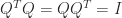 (the identity matrix). Equivalently,
  . The columns of an orthogonal matrix are orthonormal, that is, they have 2-norm (Euclidean length)
  rotation matrix has the form
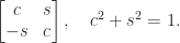
 and
and  for some
  , and the multiplication
  for a
for a  vector
  , such a matrix has the form
 Householder reflector corresponding to
 ![v = [1,1,1,1]^T/2](https://s0.wp.com/latex.php?latex=v+%3D+%5B1%2C1%2C1%2C1%5D%5ET%2F2&bg=ffffff&fg=222222&s=0&c=20201002) :
:![\frac{1}{2} \left[\begin{array}{@{\mskip2mu}rrrr@{\mskip2mu}} 1 & -1 & -1 & -1\\ -1 & 1 & -1 & -1\\ -1 & -1 & 1 & -1\\ -1 & -1 & -1 & 1\\ \end{array}\right].](https://s0.wp.com/latex.php?latex=%5Cfrac%7B1%7D%7B2%7D+++++++++%5Cleft%5B%5Cbegin%7Barray%7D%7B%40%7B%5Cmskip2mu%7Drrrr%40%7B%5Cmskip2mu%7D%7D++++++++++++++++++++++++1+%26+++-1+%26+++-1+%26+++-1%5C%5C+++++++++++++++++++++++-1+%26++++1+%26+++-1+%26+++-1%5C%5C+++++++++++++++++++++++-1+%26+++-1+%26++++1+%26+++-1%5C%5C+++++++++++++++++++++++-1+%26+++-1+%26+++-1+%26++++1%5C%5C++++++++%5Cend%7Barray%7D%5Cright%5D.+&bg=ffffff&fg=222222&s=0&c=20201002)

 for any vector
  .
. is skew-symmetric (
 ) then
  (the matrix exponential) is orthogonal and the Cayley transform
  is orthogonal as long as
  , where
  is the conjugate transpose of
  matrix
  is
is  :
:
 then
then  , so
, so  solves the equation, meaning that any 1-inverse is an equation-solving inverse. Condition (2) implies that
  if
if  .
. ).
). or
or  . For any system of linear equations
  minimizes
  and has the minimum 2–norm over all minimizers.
 is an SVD, where the
  matrix
  with
with  (so that
  ), then
 then the concise formula
  holds.
 such that
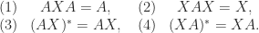
 . The first condition is the same as the second of the Moore–Penrose conditions, but the second and third have a different flavour. The index of a matrix of
  ; it is characterized as the dimension of the largest Jordan block of
  then
then  . The Drazin inverse is an equation-solving inverse precisely when
  , for then
  , which is the first of the Moore–Penrose conditions.
 and
and  has only zero eigenvalues, then
![A = \left[\begin{array}{rrr} 1 & -1 & -1\\[3pt] 0 & 0 & -1\\[3pt] 0 & 0 & 0 \end{array}\right], \quad A^+ = \left[\begin{array}{rrr} \frac{1}{2} & -\frac{1}{2} & 0\\[3pt] -\frac{1}{2} & \frac{1}{2} & 0\\[3pt] 0 & -1 & 0 \end{array}\right], \quad A^D = \left[\begin{array}{rrr} 1 & -1 & 0\\[3pt] 0 & 0 & 0\\[3pt] 0 & 0 & 0 \end{array}\right].](https://s0.wp.com/latex.php?latex=A+%3D+%5Cleft%5B%5Cbegin%7Barray%7D%7Brrr%7D+1+%26+-1+%26+-1%5C%5C%5B3pt%5D+0+%26+0+%26+-1%5C%5C%5B3pt%5D+0+%26+0+%26+0+%5Cend%7Barray%7D%5Cright%5D%2C+%5Cquad+A%5E%2B+%3D+%5Cleft%5B%5Cbegin%7Barray%7D%7Brrr%7D+%5Cfrac%7B1%7D%7B2%7D+%26+-%5Cfrac%7B1%7D%7B2%7D+%26+0%5C%5C%5B3pt%5D+-%5Cfrac%7B1%7D%7B2%7D+%26+%5Cfrac%7B1%7D%7B2%7D+%26+0%5C%5C%5B3pt%5D+0+%26+-1+%26+0+%5Cend%7Barray%7D%5Cright%5D%2C+%5Cquad+A%5ED+%3D+%5Cleft%5B%5Cbegin%7Barray%7D%7Brrr%7D+1+%26+-1+%26+0%5C%5C%5B3pt%5D+0+%26+0+%26+0%5C%5C%5B3pt%5D+0+%26+0+%26+0+%5Cend%7Barray%7D%5Cright%5D.+&bg=ffffff&fg=222222&s=0&c=20201002)
