Seven Sins of Numerical Linear Algebra

In numerical linear algebra we are concerned with solving linear algebra problems accurately and efficiently and understanding the sensitivity of the problems to perturbations. We describe seven sins, whereby accuracy or efficiency is lost or misleading information about sensitivity is obtained.

1. Inverting a Matrix

In linear algebra courses we learn that the solution to a linear system $Ax = b$ of $n$ equations in $n$ unknowns can be written $x = A^{-1}b$ , where $A^{-1}$ is the matrix inverse. What is not always emphasized is that there are very few circumstances in which one should compute $A^{-1}$ . Indeed one would not solve the scalar ( $n=1$ ) system $7x = 21$ by computing $x = 7^{-1} \times 21$ , but rather would carry out a division $x = 21/7$ . In the $n\times n$ case, it is faster and more accurate to solve a linear system by LU factorization (Gaussian elimination) with partial pivoting than by inverting $A$ (which has, in any case, to be done by LU factorization).

Rare cases where $A^{-1}$ is required are in statistics, where the diagonal elements of the inverse of the covariance matrix are relevant quantities, and in certain algorithms for computing matrix functions.

2. Forming the Cross-Product Matrix A^TA

The solution to the linear least squares problem $\min_x\| b - Ax \|_2$ , where $A$ is a full-rank $m\times n$ matrix with $m\ge n$ , satisfies the normal equations $A^T\!A x = A^Tb$ . It is therefore natural to form the symmetric positive definite matrix $A^T\!A$ and solve the normal equations by Cholesky factorization. While fast, this method is numerically unstable when $A$ is ill conditioned. By contrast, solving the least squares problem via QR factorization is always numerically stable.

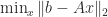
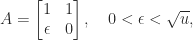
What is wrong with the cross-product matrix $A^T\!A$ (also known as the Gram matrix)? It squares the data, which can cause a loss of information in floating-point arithmetic. For example, if

$A = \begin{bmatrix} 1 & 1 \\ \epsilon & 0 \end{bmatrix}, \quad 0 < \epsilon < \sqrt{u},$

where $u$ is the unit roundoff of the floating point arithmetic, then

$A^T\!A = \begin{bmatrix} 1 + \epsilon^2 & 1 \\ 1 & 1 \end{bmatrix}$

is positive definite but, since $\epsilon^2<u$ , in floating-point arithmetic $1+\epsilon^2$ rounds to $1$ and so

$\mathrm{f\kern.2ptl}( A^T\!A) = \begin{bmatrix} 1 & 1 \\ 1 & 1 \end{bmatrix}.$

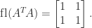
which is singular, and the information in $\epsilon$ has been lost.

Another problem with the cross product matrix is that the $2$ -norm condition number of $A^T\!A$ is the square of that of $A$ , and this leads to numerical instability in algorithms that work with $A^T\!A$ when the condition number is large.

3. Evaluating Matrix Products in an Inefficient Order

The cost of evaluating a matrix product depends on the order in which the product is evaluated (assuming the matrices are not all $n\times n$ ). More precisely, matrix multiplication is associative, so $A(BC) = (AB)C$ , and in general the cost of the evaluation of a product depends on where one puts the parentheses. One order may be much superior to others, so one should not simply evaluate the product in a fixed left-right or right-left order. For example, if $x$ , $y$ , and $z$ are $n$ -vectors then $xy^Tz$ can be evaluated as

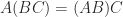
$(xy^T)z$ : a vector outer product followed by a matrix–vector product, costing $O(n^2)$ operations, or
$x (y^Tz)$ : a vector scalar product followed by a vector scaling, costing just $O(n)$ operations.

In general. finding where to put the parentheses in a matrix product $A_1A_2\dots A_k$ in order to minimize the operation count is a difficult problem, but for many cases that arise in practice it is easy to determine a good order.

4. Assuming that a Matrix is Positive Definite

Symmetric positive definite matrices (symmetric matrices with positive eigenvalues) are ubiquitous, not least because they arise in the solution of many minimization problems. However, a matrix that is supposed to be positive definite may fail to be so for a variety of reasons. Missing or inconsistent data in forming a covariance matrix or a correlation matrix can cause a loss of definiteness, and rounding errors can cause a tiny positive eigenvalue to go negative.

Definiteness implies that

the diagonal entries are positive,
$\det(A) > 0$ ,
$|a_{ij}| < \sqrt{a_{ii}a_{jj}}$ for all $i \ne j$ ,

but none of these conditions, or even all taken together, guarantees that the matrix has positive eigenvalues.

The best way to check definiteness is to compute a Cholesky factorization, which is often needed anyway. The MATLAB function chol returns an error message if the factorization fails, and a second output argument can be requested, which is set to the number of the stage on which the factorization failed, or to zero if the factorization succeeded. In the case of failure, the partially computed $R$ factor is returned in the first argument, and it can be used to compute a direction of negative curvature (as needed in optimization), for example.

This sin takes the top spot in Schmelzer and Hauser’s Seven Sins in Portfolio Optimization, because in portfolio optimization a negative eigenvalue in the covariance matrix can identify a portfolio with negative variance, promising an arbitrarily large investment with no risk!

5. Not Exploiting Structure in the Matrix

One of the fundamental tenets of numerical linear algebra is that one should try to exploit any matrix structure that might be present. Sparsity (a matrix having a large number of zeros) is particularly important to exploit, since algorithms intended for dense matrices may be impractical for sparse matrices because of extensive fill-in (zeros becoming nonzero). Here are two examples of structures that can be exploited.

Matrices from saddle point problems are symmetric indefinite and of the form

$\notag C = \begin{bmatrix} A & B^T \\ B & 0 \end{bmatrix},$

with $A$ symmetric positive definite. Much work has been done on developing numerical methods for solving $Cx = b$ that exploit the block structure and possible sparsity in $A$ and $B$ . A second example is a circulant matrix

$\notag C = \begin{bmatrix} c_1 & c_2 & \dots & c_n \\ c_n & c_1 & \dots & \vdots \\ \vdots & \ddots & \ddots & c_2 \\ c_2 & \dots & c_n & c_1 \\ \end{bmatrix}.$

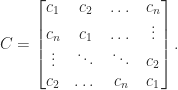
Circulant matrices have the important property that they are diagonalized by a unitary matrix called the discrete Fourier transform matrix. Using this property one can solve $Cx = v$ in $O(n \log_2n)$ operations, rather than the $O(n^3)$ operations required if the circulant structure is ignored.

Ideally, linear algebra software would detect structure in a matrix and call an algorithm that exploits that structure. A notable example of such a meta-algorithm is the MATLAB backslash function x = A\b for solving $Ax = b$ . Backslash checks whether the matrix is triangular (or a permutation of a triangular matrix), upper Hessenberg, symmetric, or symmetric positive definite, and applies an appropriate method. It also allows $A$ to be rectangular and solves the least squares problem if there are more rows than columns and the underdetermined system if there are more columns than rows.

6. Using the Determinant to Detect Near Singularity

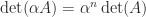
An $n\times n$ matrix $A$ is nonsingular if and only if its determinant is nonzero. One might therefore expect that a small value for $\det(A)$ indicates a matrix that is nearly singular. However, the size of $\det(A)$ tells us nothing about near singularity. Indeed, since $\det(\alpha A) = \alpha^n \det(A)$ we can achieve any value for the determinant by multiplying by a scalar $\alpha$ , yet $\alpha A$ is no more or less nearly singular than $A$ for $\alpha \ne 0$ .

Another limitation of the determinant is shown by the two matrices

$\notag T = \begin{bmatrix} 1 & -1 & -1 & \dots & -1\\ & 1 & -1 & \dots & -1\\ & & 1 & \dots & \vdots\\ & & & \ddots & -1 \\ & & & & 1 \end{bmatrix}, \quad U = \begin{bmatrix} 1 & 1 & 1 & \dots & 1\\ & 1 & 1 & \dots & 1\\ & & 1 & \dots & \vdots\\ & & & \ddots & 1 \\ & & & & 1 \end{bmatrix} \qquad (1)$

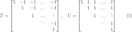
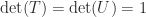
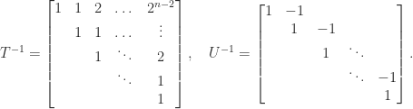
Both matrices have unit diagonal and off-diagonal elements bounded in modulus by $1$ . So $\det(T) = \det(U) = 1$ , yet

$\notag T^{-1} = \begin{bmatrix} 1 & 1 & 2 & \dots & 2^{n-2}\\ & 1 & 1 & \dots & \vdots\\ & & 1 & \ddots & 2\\ & & & \ddots & 1 \\ & & & & 1 \end{bmatrix}, \quad U^{-1} = \begin{bmatrix} 1 & -1 & & & \\ & 1 & -1 & & \\ & & 1 & \ddots & \\ & & & \ddots & -1 \\ & & & & 1 \end{bmatrix}.$

So $T$ is ill conditioned for large $n$ . In fact, if we change the $(n,1)$ element of $T$ to $-2^{n-2}$ then the matrix becomes singular! By contrast, $U$ is always very well conditioned. The determinant cannot distinguish between the ill-conditioned $T$ and the well-conditioned $U$ .

7. Using Eigenvalues to Estimate Conditioning

For any $n\times n$ matrix $A$ and any consistent matrix norm it is true that $\|A\| \ge |\lambda_i|$ for all $i$ , where the $\lambda_i$ are the eigenvalue of $A$ . Since the eigenvalues of $A^{-1}$ are $\lambda^{-1}$ , it follows that the matrix condition number $\kappa(A) = \|A\| \, \|A^{-1}\|$ is bounded below by the ratio of largest to smallest eigenvalue in absolute value, that is,

$\notag \kappa(A) \ge \displaystyle\frac{ \max_i |\lambda_i| } { \min_i |\lambda_i| }.$

But as the matrix $T$ in (1) shows, this bound can be very weak.

It is singular values not eigenvalues that characterize the condition number for the 2-norm. Specifically,

$\notag \kappa_2(A) = \displaystyle\frac{\sigma_1}{\sigma_n},$

where $A = U\Sigma V^T$ is a singular value decomposition (SVD), with $U$ and $V$ orthogonal and $\Sigma = \mathrm{diag}(\sigma_i)$ , $\sigma_1 \ge \sigma_2 \ge \cdots \ge \sigma_n \ge 0$ . If $A$ is symmetric, for example, then the sets $\{ |\lambda_i| \}$ and $\{\sigma_i \}$ are the same, but in general the eigenvalues $\lambda_i$ and singular values $\sigma_i$ can be very different.

Seven Sins of Numerical Linear Algebra

1. Inverting a Matrix

2. Forming the Cross-Product Matrix A^TA

3. Evaluating Matrix Products in an Inefficient Order

4. Assuming that a Matrix is Positive Definite

5. Not Exploiting Structure in the Matrix

6. Using the Determinant to Detect Near Singularity

7. Using Eigenvalues to Estimate Conditioning

Related Blog Posts

One thought on “Seven Sins of Numerical Linear Algebra”

Leave a reply to Andreas Varga Cancel reply

1. Inverting a Matrix

2. Forming the Cross-Product Matrix A^TA

3. Evaluating Matrix Products in an Inefficient Order

4. Assuming that a Matrix is Positive Definite

5. Not Exploiting Structure in the Matrix

6. Using the Determinant to Detect Near Singularity

7. Using Eigenvalues to Estimate Conditioning

Related Blog Posts

Share this:

Related

One thought on “Seven Sins of Numerical Linear Algebra”

Leave a reply to Andreas Varga Cancel reply