I thought it would be useful to provide my own MATLAB function nearcorr.m implementing the alternating projections algorithm. The listing is below. To see how it compares with the NAG code g02aa.m I ran the test code
%NEARCORR_TEST  Compare g02aa and nearcorr.

rng(10)                                  % Seed random number generators.
n = 100;
A = gallery('randcorr',n);               % Random correlation matrix.
E  = randn(n)*1e-1;  A = A + (E + E')/2; % Perturb it.
tol = 1e-10;

% A = cor1399; tol = 1e-4;

fprintf('g02aa:\n')
maxits = int64(-1);  % For linear equation solver.
maxit = int64(-1);   % For Newton iteration.
tic
[~,X1,iter1,feval,nrmgrd,ifail] = g02aa(A,'errtol',tol,'maxits',maxits, ...
                                          'maxit',maxit);
toc

fprintf('  Newton steps taken: %d\n', iter1);
fprintf('  Norm of gradient of last Newton step: %6.4f\n', nrmgrd);
if ifail > 0, fprintf('  g02aa failed with ifail = %g\n', ifail), end

fprintf('nearcorr:\n')
tic
[X2,iter2] = nearcorr(A,tol,[],[],[],[],1);
toc
fprintf('  Number of iterations: %d\n', iter2);

fprintf('  Normwise relative difference between computed solutions:')
fprintf('%9.2e\n', norm(X1-X2,1)/norm(X1,1))
Running under Windows 7 on an Ivy Bridge Core i7 processor @4.4Ghz I obtained the following results, where the “real-life” matrix is based on stock data:
| Matrix |
Code |
Time (secs) |
Iterations |
| 1. Random (100), tol = 1e-10 |
g02aa |
0.023 |
4 |
|
nearcorr |
0.052 |
15 |
| 2. Random (500), tol = 1e-10 |
g02aa |
0.48 |
4 |
|
nearcorr |
3.01 |
26 |
| 3. Real-life (1399), tol = 1e-4 |
g02aa |
6.8 |
5 |
|
nearcorr |
100.6 |
68 |
The results show that while nearcorr can be fast for small dimensions, the number of iterations, and hence its run time, tends to increase with the dimension and it can be many times slower than the Newton method. This is a stark illustration of the difference between quadratic convergence and linear (with problem-dependent constant) convergence. Here is my MATLAB function nearcorr.m.
function [X,iter] = nearcorr(A,tol,flag,maxits,n_pos_eig,w,prnt)
%NEARCORR    Nearest correlation matrix.
%   X = NEARCORR(A,TOL,FLAG,MAXITS,N_POS_EIG,W,PRNT)
%   finds the nearest correlation matrix to the symmetric matrix A.
%   TOL is a convergence tolerance, which defaults to 16*EPS.
%   If using FLAG == 1, TOL must be a 2-vector, with first component
%   the convergence tolerance and second component a tolerance
%   for defining "sufficiently positive" eigenvalues.
%   FLAG = 0: solve using full eigendecomposition (EIG).
%   FLAG = 1: treat as "highly non-positive definite A" and solve
%             using partial eigendecomposition (EIGS).
%   MAXITS is the maximum number of iterations (default 100, but may
%   need to be increased).
%   N_POS_EIG (optional) is the known number of positive eigenvalues of A.
%   W is a vector defining a diagonal weight matrix diag(W).
%   PRNT = 1 for display of intermediate output.

%   By N. J. Higham, 13/6/01, updated 30/1/13, 15/11/14, 07/06/15.
%   Reference:  N. J. Higham, Computing the nearest correlation
%   matrix---A problem from finance. IMA J. Numer. Anal.,
%   22(3):329-343, 2002.

if ~isequal(A,A'), error('A must by symmetric.'), end
if nargin < 2 || isempty(tol), tol = length(A)*eps*[1 1]; end
if nargin < 3 || isempty(flag), flag = 0; end
if nargin < 4 || isempty(maxits), maxits = 100; end
if nargin < 6 || isempty(w), w = ones(length(A),1); end
if nargin < 7, prnt = 1; end

n = length(A);
if flag >= 1
   if nargin < 5 || isempty(n_pos_eig)
      [V,D] = eig(A); d = diag(D);
      n_pos_eig = sum(d >= tol(2)*d(n));
   end
   if prnt, fprintf('n = %g, n_pos_eig = %g\n', n, n_pos_eig), end
end

X = A; Y = A;
iter = 0;
rel_diffX = inf; rel_diffY = inf; rel_diffXY = inf;
dS = zeros(size(A));

w = w(:); Whalf = sqrt(w*w');

while max([rel_diffX rel_diffY rel_diffXY]) > tol(1)

   Xold = X;
   R = Y - dS;
   R_wtd = Whalf.*R;
   if flag == 0
      X = proj_spd(R_wtd);
   elseif flag == 1
      [X,np] = proj_spd_eigs(R_wtd,n_pos_eig,tol(2));
   end
   X = X ./ Whalf;
   dS = X - R;
   Yold = Y;
   Y = proj_unitdiag(X);
   rel_diffX = norm(X-Xold,'fro')/norm(X,'fro');
   rel_diffY = norm(Y-Yold,'fro')/norm(Y,'fro');
   rel_diffXY = norm(Y-X,'fro')/norm(Y,'fro');
   iter = iter + 1;
   if prnt
      fprintf('%2.0f:  %9.2e  %9.2e  %9.2e', ...
               iter, rel_diffX, rel_diffY, rel_diffXY)
      if flag >= 1, fprintf('  np = %g\n',np), else fprintf('\n'), end
   end
   if iter > maxits
       error(['Stopped after ' num2str(maxits) ' its. Try increasing MAXITS.'])
   end

end

%%%%%%%%%%%%%%%%%%%%%%%%
function A = proj_spd(A)
%PROJ_SPD

if ~isequal(A,A'), error('Not symmetric!'), end
[V,D] = eig(A);
A = V*diag(max(diag(D),0))*V';
A = (A+A')/2; % Ensure symmetry.

%%%%%%%%%%%%%%%%%%%%%%%%%%%%%%%%%%%%%%%%%%%%%%%%%%%%%%%%%%%%%
function [A,n_pos_eig_found] = proj_spd_eigs(A,n_pos_eig,tol)
%PROJ_SPD_EIGS

if ~isequal(A,A'), error('Not symmetric!'), end
k = n_pos_eig + 10; % 10 is safety factor.
if k > length(A), k = n_pos_eig; end
opts.disp = 0;
[V,D] = eigs(A,k,'LA',opts); d = diag(D);
j = (d > tol*max(d));
n_pos_eig_found = sum(j);
A = V(:,j)*D(j,j)*V(:,j)';  % Build using only the selected eigenpairs.
A = (A+A')/2; % Ensure symmetry.

%%%%%%%%%%%%%%%%%%%%%%%%%%%%%
function A = proj_unitdiag(A)
%PROJ_SPD

n = length(A);
A(1:n+1:n^2) = 1;
Updates
- Links updated August 4, 2014.
nearcorr.m corrected November 15, 2014: iter was incorrectly initialized (thanks to Mike Croucher for pointing this out).- Added link to Mike Croucher’s Python alternating directions code, November 17, 2014.
- Corrected an error in the convergence test, June 7, 2015. Effect on performance will be minimal (thanks to Nataša Strabić for pointing this out).


 , instead of bounding the
  th term
  by
by  , a potentially smaller bound is used.
  and are not willing to compute
  but are willing to compute lower powers of
  . We have
  , so
, so  ,
,  ,
,  , and
, and  . But it is easy to see that
 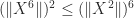 and
and 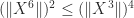 , so we can discard two of the bounds, ending up with
 for values of
  up to some small, fixed value. The gains can be significant. Consider the matrix
 , but
, but 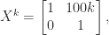
 , which is a significant improvement.
 is the spectral radius (the largest modulus of any eigenvalue). The upper bound corresponds to the usual analysis. The lower bound is something that we cannot use to bound the norm of the power series. The middle term is what we are using, and as
  the middle term converges to the lower bound, which can be arbitrarily smaller than the upper bound.
 I learned about Anderson acceleration in the minisymposium
  authors listed alphabetically, and it is assumed that the paper is from a community where it is the custom to order authors alphabetically.
 coauthors are chosen independently at random they will all have surnames later in the alphabet than the first author. This definition is not precise, since it is not clear what is the sample space of all possible names, so it is better to regard the spotlight factor as being defined by the formula given by Tompa, which is implemented in the MATLAB function below.
 be an
be an  real or complex matrix. Consider the principal logarithm—the one for which
  has imaginary part in
 ![(-\pi,\pi]](https://s0.wp.com/latex.php?latex=%28-%5Cpi%2C%5Cpi%5D&bg=ffffff&fg=222222&s=0&c=20201002) —and define
—and define  for
for  (an important special case being
  for an integer
  for all
  for all
  whenever
  commute.
 is always true.
 is false.
 and a power
  in the above expressions stands for the families of all possible logarithms and powers then the identities are all true. But from a computational viewpoint we are usually concerned with a particular branch of each function, the principal branch, so equality cannot be taken for granted.
 , and it arises from the scalar unwinding number introduced by Corless, Hare and Jeffrey in 1996
 , so the relation in the first quiz question is clearly valid when
  , which is the case when the eigenvalues of
 and the matrix
  has eigenvalues with imaginary parts in
  ? The following incomplete MATLAB code implements the Schur algorithm developed in the paper. The

