Randsvd Matrices with Large Growth Factors

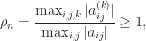
Sixty years ago James Wilkinson published his backward error analysis of Gaussian elimination for solving a linear system $Ax = b$ , where $A$ is a nonsingular $n\times n$ matrix. He showed that in floating-point arithmetic the computed solution $\widehat{x}$ satisfies

$(A+\Delta A) \widehat{x} = b, \qquad \|\Delta A\|_{\infty} \le p(n) \rho_n u \|A\|_{\infty},$

where $u$ is the unit roundoff and $p$ is a low degree polynomial. The term $\rho_n$ is the growth factor, defined by

$\rho_n = \displaystyle\frac{\max_{i,j,k} |a_{ij}^{(k)}|} {\max_{i,j}|a_{ij}|} \ge 1,$

where the $a_{ij}^{(k)}$ are the elements at the $k$ th stage of Gaussian elimination. The growth factor measures how much elements grow during the elimination. We would like the product $p(n)\rho_n$ to be of order 1, so that $\Delta A$ is a small relative perturbation of $A$ . We therefore need $\rho_n$ not to be too large.

With partial pivoting, in which row interchanges are used to ensure that at each stage the pivot element is the largest in its column, Wilkinson showed that $\rho_n \le 2^{n-1}$ and that equality is possible. Such exponential growth implies a large $\Delta A$ (unless we are lucky), meaning a severe loss of numerical stability. However, seventy years of digital computing experience have shown that $\rho_n$ is usually of modest size in practice. Explaining why this is the case is one of the outstanding problems in numerical analysis.

It is easy to experiment with growth factors in MATLAB. I will use the function

function g = gf(A)
%GF     Approximate growth factor.
%   g = GF(A) is an approximation to the
%   growth factor for LU factorization
%   with partial pivoting.
[~,U] = lu(A);
g = max(abs(U),[],'all')/max(abs(A),[],'all');

It computes a lower bound on the growth factor (since it only considers $k=n$ in the numerator in the definition), but it is entirely adequate for our purposes here. Let’s compute the growth factor for a random matrix of order 10,000 with elements from the standard normal distribution (mean 0, variance 1):

>> rng(1); n = 10000; gf(randn(n))
ans =
6.1335e+01

Growth of 61 is unremarkable for a matrix of this size. Now we try a matrix of the same size generated by the gallery('randsvd') function:

>> A = gallery('randsvd',n,1e6,2,[],[],1);
>> gf(A)
ans =
9.7544e+02

This function generates an $n\times n$ matrix with known singular value distribution and with singular vector matrices that are random orthogonal matrices from the Haar distribution. The parameter 1e6 specifies the 2-norm condition number, while the 2 (the mode parameter) specifies that there is only one small singular value, so the singular values are 1 repeated $n-1$ times and 1e-6. Growth of 975 is exceptional! These matrices have been in MATLAB since the 1990s, but this large growth property has apparently not been noticed before.

It turns out that mode 2 randsvd matrices generate with high probability growth factors of size at least $n/(4 \log n)$ for any condition number and for any pivoting strategy, not just partial pivoting. One way to check this is to randomly permute the columns of $A$ before doing the LU factorization with partial pivoting:

>> gf(A(:,randperm(n)))
ans =
7.8395e+02

Here is a plot showing the maximum over 12 randsvd matrices for each $n$ of the growth factors for three different pivoting strategies, along with the maximum growth factors for partial pivoting for rand and randn matrices. The black curve is $n/(4 \log n)$ . This plot emphasizes the unusually large growth for mode 2 randsvd matrices.

What is the explanation for this large growth? It stems from three facts.

Haar distributed orthogonal matrices have the property that that their elements are fairly small with high probability, as shown by Jiang in 2005.
If the largest entries in magnitude of $A$ and $A^{-1}$ are both small, in the sense that their product is $\theta \ll 1$ , then $A$ will produce a growth factor of at least $1/\theta$ for any pivoting strategy. This was proved by Des Higham and I in the paper Large Growth Factors in Gaussian Elimination with Pivoting.
If $W$ is an orthogonal matrix generating large growth then a rank-1 perturbation of 2-norm at most 1 tends to preserve the large growth.

For full details see the new EPrint Random Matrices Generating Large Growth in LU Factorization with Pivoting by Des Higham, Srikara Pranesh and me.

Is growth of order $n$ a problem in practice? It can be for two reasons.

The largest dense linear systems $Ax = b$ solved today are of dimension $n = 10^7$ . If we work in single precision then $nu \approx 1$ and so LU factorization can potentially be completely unstable if there is growth of order $n$ .
For IEEE half precision arithmetic growth of order $n$ will cause overflow once $n$ exceeds $10^5 / \max_{i,j} |a_{ij}|$ . It was overflow in half precision LU factorization on randsvd matrices that alerted us to the large growth.

Singular Values of Rank-1 Perturbations of an Orthogonal Matrix

What effect does a rank-1 perturbation of norm 1 to an $n\times n$ orthogonal matrix have on the extremal singular values of the matrix? Here, and throughout this post, the norm is the 2-norm. The largest singular value of the perturbed matrix is bounded by $2$ , as can be seen by taking norms, so let us concentrate on the smallest singular value.

Consider first a perturbation of the identity matrix: $B = I + xy^T$ , for unit norm $x$ and $y$ . The matrix $B$ has eigenvalues 1 (repeated $n-1$ times) and $1 + y^Tx$ . The matrix is singular—and hence has a zero singular value—precisely when $y^Tx = -1$ , which is the smallest value that the inner product $y^Tx$ can take.

Another example is $B = A + yy^T$ , where $A = I - 2yy^T$ and $y$ has unit norm, so that $A$ is a Householder matrix. Here, $B = I - yy^T$ is singular with null vector $y$ , so it has a zero singular value,

Let’s take a random orthogonal matrix and perturb it with a random rank-1 matrix of unit norm. We use the following MATLAB code.

n = 100; rng(1)
A = gallery('qmult',n); % Random Haar distrib. orthogonal matrix.
x = randn(n,1); y = randn(n,1);
x = x/norm(x); y = y/norm(y);
B = A + x*y';
svd_B = svd(B);
max_svd_B = max(svd_B), min_svd_B = min(svd_B)

The output is

max_svd_B =
1.6065e+00
min_svd_B =
6.0649e-01

We started with a matrix having singular values all equal to 1 and now have a matrix with largest singular value a little larger than 1 and smallest singular value a little smaller than 1. If we keep running this code the extremal singular values of $B$ do not change much; for example, the next run gives

max_svd_B =
1.5921e+00
min_svd_B =
5.9213e-01

A rank-1 perturbation of unit norm could make $A$ singular, as we saw above, but our random perturbations are producing a well conditioned matrix.

What is the explanation? First, note that a rank-1 perturbation to an orthogonal matrix $A$ can only change two of the singular values, because the singular values are the square roots of the eigenvalues of $A^T A$ , which is the identity plus a rank- $2$ matrix. So $n-2$ singular values remain at 1.

A result of Benaych-Georges and Nadakuditi (2012) says that for large $n$ the largest and smallest singular values of $B$ tend to $(1+\sqrt{5})/2 = 1.618\dots$ and $(-1+\sqrt{5})/2 = 0.618\dots$ respectively! As our example shows, $n$ does not have to be large for these limits to be approximations correct to roughly the first digit.

The result in question requires the original orthogonal matrix to be from the Haar distribution, and such matrices can be generated by A = gallery('qmult',n) or by the construction

[Q,R] = qr(randn(n));
Q = Q*diag(sign(diag(R)));

(See What Is a Random Orthogonal Matrix?.) The result also requires $u$ and $v$ to be unit-norm random vectors with independent entries from the same distribution.

However, as the next example shows, the perturbed singular values can be close to the values that the Benaych-Georges and Nadakuditi result predicts even when the conditions of the result are violated:

n = 100; rng(1)
A = gallery('orthog',n);   % Random orthogonal matrix (not Haar).
x = rand(n,1); y = (1:n)'; % Non-random y.
x = x/norm(x); y = y/norm(y);
B = A + x*y';
svd_B = svd(B);
max_svd_B = max(svd_B), min_svd_B = min(svd_B)

max_svd_B =
1.6069e+00
min_svd_B =
6.0687e-01

The question of the conditioning of a rank-1 perturbation of an orthogonal matrix arises in the recent EPrint Random Matrices Generating Large Growth in LU Factorization with Pivoting.

Accurately Computing the Softmax Function

The softmax function takes as input an $n$ -vector $x$ and returns a vector $g(x)$ with elements

$g_j(x) = \displaystyle\frac{\mathrm{e}^{x_j}}{\sum_{i=1}^n \mathrm{e}^{x_i}}, \quad j=1\colon n,$

The elements of $g$ are all between $0$ and $1$ and they sum to 1, so $g$ can be regarded as a vector of probabilities. Softmax is a key function in machine learning algorithms.

Softmax is the gradient vector of the log-sum-exp function

$f(x) = \displaystyle\log \sum_{i=1}^n \mathrm{e}^{x_i}.$

This function is an approximation to the largest element, $x_{\max} = \max_i x_i$ of the vector $x$ , as it lies between $x_{\max}$ and $x_{\max} + \log n$ .

A problem with numerical evaluation of log-sum-exp and softmax is that overflow is likely even for quite modest values of $x_i$ because of the exponentials, even though $g(x)$ cannot overflow and $f(x)$ is very unlikely to do so.

A standard solution it to incorporate a shift, $a$ , and use the formulas

$f(x) = a + \displaystyle\log \sum_{i=1}^n \mathrm{e}^{x_i-a}, \hspace*{4.5cm}(1)$

and

$g_j(x) = \displaystyle\frac{\mathrm{e}^{x_j-a}}{\sum_{i=1}^n \mathrm{e}^{x_i-a}}, \quad j=1\colon n, \hspace*{3.3cm}(2)$

where $a$ is usually set to $x_{\max}$ .

Another formula for softmax is obtained by moving the denominator into the numerator:

$g_j(x) = \exp\left(x_j - a - \log\displaystyle\sum_{i=1}^n\mathrm{e}^{x_i -a}\right). \hspace*{2cm}(3)$

This formulas is used in various codes, including in the SciPy 1.4.1 function softmax.

How accurate are these formulas when evaluated in floating-point arithmetic? To my knowledge, this question has not been addressed in the literature, but it is particularly important given the growing use of low precision arithmetic in machine learning. Two questions arise. First, is there any difference between the accuracy of the formulas (2) and (3) for $g_j(x)$ ? Second, in (1) and (3), $a$ is added to a nonnegative log term, so when $a = x_{\max}$ is negative can there be damaging subtractive cancellation?

In a recent EPrint with Pierre Blanchard and Des Higham I have investigated these questions using rounding error analysis and analysis of the conditioning of the log-sum-exp and softmax problems. In a nutshell, our findings are that while cancellation can happen, it is not a problem: the shifted formulas (1) and (2) can be safely used.

However, the alternative softmax formula (3) is not recommended, as its rounding error bounds are larger than for (2) and we have found it to produce larger errors in practice.

Here is an example from training an artificial neural network using the MATLAB Deep Learning Toolbox. The network is trained to classify handwritten digits from the widely used MNIST data set. The following figure shows the sum of the computed elements of the softmax vector $g(x)$ for 2000 vectors extracted from the training data, where $g(x)$ was computed in IEEE half precision arithmetic. The sum should be 1. The red circles are for formula (2) and the blue crosses are for the division-free formula (3). Clearly, (2) gives a better approximation to a vector of probabilities (in the sense of respecting the constraint that probabilities sum to unity); the actual errors in each vector component are also smaller for (2).

Half Precision Arithmetic: fp16 Versus bfloat16

The 2008 revision of the IEEE Standard for Floating-Point Arithmetic introduced a half precision 16-bit floating point format, known as fp16, as a storage format. Various manufacturers have adopted fp16 for computation, using the obvious extension of the rules for the fp32 (single precision) and fp64 (double precision) formats. For example, fp16 is supported by the NVIDIA P100 and V100 GPUs and the AMD Radeon Instinct MI25 GPU, as well as the A64FX Arm processor that will power the Fujitsu Post-K exascale computer.

Bfloat16

Fp16 has the drawback for scientific computing of having a limited range, its largest positive number being $6.55 \times 10^4$ . This has led to the development of an alternative 16-bit format that trades precision for range. The bfloat16 format is used by Google in its tensor processing units. Intel, which plans to support bfloat16 in its forthcoming Nervana Neural Network Processor, has recently (November 2018) published a white paper that gives a precise definition of the format.

The allocation of bits to the exponent and significand for bfloat16, fp16, and fp32 is shown in this table, where the implicit leading bit of a normalized number is counted in the significand.

Format	Significand	Exponent
bfloat16	8 bits	8 bits
fp16	11 bits	5 bits
fp32	24 bits	8 bits

Bfloat16 has three fewer bits in the significand than fp16, but three more in the exponent. And it has the same exponent size as fp32. Consequently, converting from fp32 to bfloat16 is easy: the exponent is kept the same and the significand is rounded or truncated from 24 bits to 8; hence overflow and underflow are not possible in the conversion.

On the other hand, when we convert from fp32 to the much narrower fp16 format overflow and underflow can readily happen, necessitating the development of techniques for rescaling before conversion—see the recent EPrint Squeezing a Matrix Into Half Precision, with an Application to Solving Linear Systems by me and Sri Pranesh.

The drawback of bfloat16 is its lesser precision: essentially 3 significant decimal digits versus 4 for fp16. The next table shows the unit roundoff $u$ , smallest positive (subnormal) number xmins, smallest normalized positive number xmin, and largest finite number xmax for the three formats.

	$u$	xmins	xmin	xmax
bfloat16	3.91e-03	(*)	1.18e-38	3.39e+38
fp16	4.88e-04	5.96e-08	6.10e-05	6.55e+04
fp32	5.96e-08	1.40e-45	1.18e-38	3.40e+38

(*) Unlike the fp16 format, Intel’s bfloat16 does not support subnormal numbers. If subnormal numbers were supported in the same way as in IEEE arithmetic, xmins would be 9.18e-41.

The values in this table (and those for fp64 and fp128) are generated by the MATLAB function float_params that I have made available on GitHub and at MathWorks File Exchange.

Harmonic Series

An interesting way to compare these different precisions is in summation of the harmonic series $1 + 1/2 + 1/3 + \cdots$ . The series diverges, but when summed in the natural order in floating-point arithmetic it converges, because the partial sums grow while the addends decrease and eventually the addend is small enough that it does not change the partial sum. Here is a table showing the computed sum of the harmonic series for different precisions, along with how many terms are added before the sum becomes constant.

Arithmetic	Computed Sum	Number of terms
bfloat16	$5.0625$	$65$
fp16	$7.0859$	$513$
fp32	$15.404$	$2097152$
fp64	$34.122$	$2.81\dots\times 10^{14}$

The differences are striking! I determined the first three values in MATLAB. The fp64 value is reported by Malone based on a computation that took 24 days, and he also gives analysis to estimate the limiting sum and corresponding number of terms for fp64.

Fused Multiply-Add

The NVIDIA V100 has tensor cores that can carry out the computation D = C + A*B in one clock cycle for 4-by-4 matrices A, B, and C; this is a 4-by-4 fused multiply-add (FMA) operation. Moreover, C and D can be in fp32. The benefits that the speed and accuracy of the tensor cores can bring over plain fp16 is demonstrated in Harnessing GPU Tensor Cores for Fast FP16 Arithmetic to Speed up Mixed-Precision Iterative Refinement Solvers.

Intel’s bfloat16 format supports a scalar FMA d = c + a*b, where c and d are in fp32.

Conclusion

A few years ago we had just single precision and double precision arithmetic. With the introduction of fp16 and fp128 in the IEEE standard in 2008, and now bfloat16 by Google and Intel, the floating-point landscape is becoming much more interesting.

How to Program log z

While Fortran was the first high-level programming language used for scientific computing, Algol 60 was the vehicle for publishing mathematical software in the early 1960s. Algol 60 had real arithmetic, but complex arithmetic had to be programmed by working with real and imaginary parts. Functions of a complex variable were not built-in, and had to be written by the programmer.

I’ve written a number of papers on algorithms to compute the (principal) logarithm of a matrix. The problem of computing the logarithm of a complex scalar—given a library routine that handles real arguments—might appear trivial, by comparison. That it is not can be seen by looking at early attempts to provide such a function in Algol 60.

The paper

J. R. Herndon (1961). Algorithm 48: Logarithm of a complex number. Comm. ACM, 4(4), 179.

presents an Algol 60 code for computing $\log z$ , for a complex number $z$ . It uses the arctan function to obtain the argument of a complex number.

The paper

A. P. Relph (1962). Certification of Algorithm 48: Logarithm of a complex number. Comm. ACM, 5(6), 347.

notes three problems with Herndon’s code: it fails for $z$ with zero real part, the imaginary part of the logarithm is on the wrong range (it should be $(-\pi,\pi]$ for the principal value), and the code uses log (log to the base 10) instead of ln (log to the base $e$ ). The latter error suggests to me that the code had never actually been run, as for almost any argument it would produce an incorrect value. This is perhaps not surprising since Algol 60 compilers must have only just started to become available in 1961.

The paper

M. L. Johnson and W. Sangren, W. (1962). Remark on Algorithm 48: Logarithm of a complex number. Comm. CACM, 5(7), 391.

contains more discussion about avoiding division by zero and getting signs correct. In

D. S. Collens (1964). Remark on remarks on Algorithm 48: Logarithm of a complex number. Comm. ACM, 7(8), 485.

Collens notes that Johnson and Sangren’s code wrongly gives $\log 0 = 0$ and has a missing minus sign in one statement. Finally, Collens gives in

D. S. Collens (1964). Algorithm 243: Logarithm of a complex number: Rewrite of Algorithm 48. Comm. CACM, 7(11), 660.

a rewritten algorithm that fixes all the earlier errors.

So it took five papers over a three year period to produce a correct Algol 60 code for the complex logarithm! Had those authors had the benefit of today’s interactive computing environments that period could no doubt have been shortened, but working with multivalued complex functions is necessarily a tricky business, as I have explained in earlier posts here and here.

Numerical Linear Algebra Group 2017

The Manchester Numerical Linear Algebra Group (many of whom are in the October 2017 photo below) was involved in a variety of activities this year. This post summarizes what we got up to. Publications are not included here, but many of them can be found on MIMS EPrints under the category Numerical Analysis.

Software

Together with Jack Dongarra’s team at the University of Tennessee the group is one of the two partners involved in the development of PLASMA: Parallel Linear Algebra Software for Multicore Architectures.

PhD students Weijian Zhang, Steven Elsworth and Jonathan Deakin released Etymo—a search engine for machine learning research and development.

We continue to make our research codes available, which is increasingly done on GitHub; see the repositories of Fasi, Higham, Relton, Sego, Tisseur, Zhang. We also put MATLAB software on MATLAB Central File Exchange and on our own web sites, e.g., the Rational Krylov Toolbox (RKToolbox).

PhD Students

New PhD students Gian Maria Negri Porzio and Thomas McSweeney joined the group in September 2017.

Postdoctoral Research Associates (PDRAs)

Sam Relton, who was working on the Parallel Numerical Linear Algebra for Extreme Scale Systems (NLAFET) project, left in June 2017 to take up a position at the University of Leeds. Negin Bagherpour joined NLAFET in March 2017, leaving in November 2017.

Srikara Pranesh joined the project in November 2017. Pierre Blanchard joined us in October 2017 to work jointly on the ICONIC project (which started in June 2017) and NLAFET.

Presentations at Conferences and Workshops

UK and Republic of Ireland Section of SIAM Annual Meeting, University of Strathclyde, January 12, 2017: Fasi, Gwynne, Higham, Zemaityte, Zhang.

2017 Joint Mathematics Meetings, Atlanta, January 4-7, 2017: Higham.

Workshop on Matrix Equations and Tensor Techniques, Pisa, Italy, February 13-14 2017: Fasi

Due Giorni di Algebra Lineare Numerica, Como, Italy, February 16-17, 2017: Fasi

International Conference on Domain Decomposition Methods DD24, Svalbard, Norway, February 6-10, 2017: Sistek.

Workshop on Batched, Reproducible, and Reduced Precision BLAS, Atlanta, February 23-25, 2017: Hammarling, Relton.

SIAM Conference on Computational Science and Engineering, Atlanta, February 27-March 3, 2017: Relton, Zounon. See the blog posts about the meeting by Nick Higham and Sam Relton.

Mawussi talking about batched BLAS in room 204! #CSE17 #SIAMCSE17 pic.twitter.com/BPGGdsGwZ1

— Samuel Relton (@sdrelton) February 27, 2017

High Performance Computing in Science and Engineering (HPCSE) 2017, Hotel Solan, Czech Republic, May 22-25, 2017: Sistek

Advances in Data Science, Manchester, May 15-16, 2017: Zhang.

Mark Girolamj opening the @dsi_uom Data Science workshop at @msimsn pic.twitter.com/CSNNdkX1Uv

— Nick Higham (@nhigham) May 15, 2017

27th Biennial Conference on Numerical Analysis, Glasgow, June 27-30, 2017: Tisseur.

A great start to the morning after the banquet with Fran Tisseur #strathna pic.twitter.com/xHGC4jtJZL

— David Gleich (@dgleich) June 30, 2017

Householder Symposium XX on Numerical Linear Algebra, The Inn at Virginia Tech, June 18-23, 2017: Tisseur.

SIAM Annual Meeting, Pittsburgh, July 10-14, 2017: Zhang (see this SIAM News article about Weijian’s presentation). A Storify of the conference is available in PDF form.

The fastest dense SVD, presented by David Keyes #SIAMAN17 pic.twitter.com/onTwPeuVfn

— Nick Higham (@nhigham) July 10, 2017

ILAS 2017 Conference, Iowa State University, USA, July 24-28, 2017: Güttel

24th IEEE Symposium on Computer Arithmetic, London, July 24-26, 2017: Higham (see this blog post by George Constantinides).

. @nhigham gave an inspiring keynote on mixed precision algorithms. So exciting! #ARITH24 pic.twitter.com/dwWpidi2VD

— G A Constantinides (@gconstantinides) July 24, 2017

LMS-EPSRC Symposium on Model Order Reduction, Durham, UK, August 8-17, 2017: Güttel

Euro-Par 2017, 23rd International European Conference on Parallel and Distributed Computing, August 28-September 1, 2017: Zounon.

INdAM Meeting Structured Matrices in Numerical Linear Algebra: Analysis, Algorithms and Applications, Cortona, Italy, September 4-8, 2017: Fasi, Tisseur.

2017 Woudschoten Conferences, Zeist, The Netherlands, 4-6 October 2017: Tisseur.

ICERM Workshop on Recent Advances in Seismic Modeling and Inversion, Brown University, USA, November 6-10, 2017: Güttel. A video recording of this talk is available.

Conference and Workshop Organization

Güttel co-organized the SIAM UKIE Annual Meeting 2017 at the University of Strathclyde January 12, 2017 and the GAMM ANLA Workshop on High-Performance Computing at the University of Cologne, September 7-8, 2017.

The Manchester SIAM Student Chapter organized an Manchester Chapter Auto Trader Industry Problem Solving Event on February 22, 2017 and the 7th Manchester SIAM Student Chapter Conference on May 5, 2017.

The group organized three minisymposia at the SIAM Conference on Computational Science and Engineering, Atlanta, February 27-March 3, 2017:

Nick Higham and Bo T. Kågström: Parallel Numerical Linear Algebra for Extreme Scale Systems. See the blog post by Nick Higham.
Sam Relton: Recent Advances in Matrix Functions and Applications.
Mawussi Zounon and Pedro Valero-Lara: Batched Linear Algebra on Multi/Many-Core Architectures. See the blog post by Sam Relton.

Visitors

Franco Zivcovic (Università degli Studi di Trento) visited the group from September 2017-January 2018.

Knowledge Transfer

The Sabisu KTP project, which ended in December 2016, has been awarded the highest grade of “Outstanding” by the KTP Grading Panel. A new KTP project with Process Integration Ltd. is under way, led by Stefan Güttel.

The MSc project of Thomas McSweeney was sponsored by NAG and produced a code for modified Cholesky factorization that will appear in the NAG Library.

Recognition and Service

Stefan Güttel continued his terms as Secretary/Treasurer of the SIAM UKIE section and vice-chair of the GAMM Activity Group on Applied and Numerical Linear Algebra.

Nick Higham served the first year of his two-year term as President of SIAM.

Weijian Zhang was awarded a SIAM Student Travel Award to attend the SIAM Annual Meeting 2017 in Pittsburgh.

Massimiliano Fasi and Mante Zemaityte were selected to present posters at the SET for Britain 2017 competition, which took place at the House of Commons, London. Fasi’s poster was “Finding Communities in Large Signed Networks with the Weighted Geometric Mean of Laplacians” and Zemaityte’s was “A Shift-and-Invert Lanczos Algorithm for the Dynamic Analysis of Structures”.

Jakub Sistek served as treasurer of the eu-maths-in.cz Czech Network for Mathematics in Industry.

Tweets of the Year

RKToolbox version 2.7 available at https://t.co/ZMvUG6guKC — new support for AAA approximants https://t.co/cDr1OAvbVc pic.twitter.com/ap6QSZHobj

— Stefan Güttel (@guettel) November 21, 2017

Prof. Higham just delivered ‘The Rise of Multiprecision Computations’ to NAG colleagues. An excellent technical talk, thank you @nhigham pic.twitter.com/jW3Rlv2wkh

— NAG (@NAGTalk) October 4, 2017

We just included subject tags in @etymo_io. Now you can filter papers by subjects! https://t.co/oqXFKVojVs pic.twitter.com/Wgy5EHqhsr

— Weijian Zhang (@zweijian) September 24, 2017

Blog Post on Etymo “Visualizing Machine Learning Papers” https://t.co/UnBYNkwFgH

— Weijian Zhang (@zweijian) August 24, 2017

Funny Faces at the #SIAMAN17 Fellows Reception – excellent entry from Tim Kelley at (1,4) position @TheSIAMNews https://t.co/UOORkkg6sX

— Nick Higham (@nhigham) September 5, 2017

Spotted near #SIAMAN17 – a reminder where we’ll be for @ICIAMnews 2019 pic.twitter.com/DEXsmvkcG9

— Nick Higham (@nhigham) 9 July 2017

Congratulations Mary and Stefan and all the best for the future @guettel, @MaryAprahamian #WeddingDay pic.twitter.com/Ct5JlD7w8A

— Nick Higham (@nhigham) June 10, 2017

March for Science getting underway in Washington, D.C. #marchforscience pic.twitter.com/SdWGPntaQY

— Nick Higham (@nhigham) April 22, 2017

Reading @TheSIAMNews today – engrossed in great column from @nhigham and missed my train stop! https://t.co/hGhEWEomxx

— G A Constantinides (@gconstantinides) April 27, 2017

Final KTP report with @sabisu has been graded as ‘Outstanding’ by a panel of independent assessors https://t.co/OkW2qrLFsG

— Stefan Güttel (@guettel) May 18, 2017

New 94-page survey of the nonlinear eigenvalue problem by @guettel and @tisseurf in Acta Numerica https://t.co/H8iDzUYGWm pic.twitter.com/OVyZICszXW

— Nick Higham (@nhigham) May 15, 2017

Writing a Ph.D. thesis can be hard! Postdoc @sdrelton reflects on the process with 10 tips for current students https://t.co/fLLV0qdkLp

— SIAM (@TheSIAMNews) April 7, 2017

Both low and high precision become more prevalent @SIAM_UKIE pic.twitter.com/DkKDhUKr5v

— Weijian Zhang (@zweijian) January 12, 2017

The Strange Case of the Determinant of a Matrix of 1s and -1s

By Nick Higham and Alan Edelman (MIT)

In a 2005 talk the second author noted that the MATLAB det function returns an odd integer for a certain 27-by-27 matrix composed of $1$ s and $-1$ s:

>> A = edelman; % Set up the matrix.
>> format long g, format compact, det(A)
ans =
           839466457497601

However, the determinant is, from its definition, a sum of an even number (27 factorial) of odd numbers, so is even. Indeed the correct determinant is 839466457497600.

At first sight, this example is rather troubling, since while MATLAB returns an integer, as expected, it is out by $1$ . The determinant is computed as the product of the diagonal entries of the $U$ factor in the LU factorization with partial pivoting of $A$ , and these entries are not all integers. Standard rounding error analysis shows that the relative error from forming that product is bounded by $nu/(1-nu)$ , with $n=27$ , where $u \approx 1.1 \times 10^{-16}$ is the unit roundoff, and this is comfortably larger than the actual relative error (which also includes the errors in computing $U$ ) of $6 \times 10^{-16}$ . Therefore the computed determinant is well within the bounds of roundoff, and if the exact result had not been an integer the incorrect last decimal digit would hardly merit discussion.

However, this matrix has more up its sleeve. Let us compute the determinant using a different implementation of Gaussian elimination with partial pivoting, namely the function gep from the Matrix Computation Toolbox:

>> [Lp,Up,Pp] = gep(A,'p'); det(Pp)*det(Up)
ans =
           839466457497600

Now we get the correct answer! To see what is happening, we can directly form the products of the diagonal elements of the $U$ factors:

>> [L,U,P] = lu(A); 
>> d = diag(U); dp = diag(Up); 
>> rel_diff_U_diags = norm((dp - d)./d,inf)
rel_diff_U_diags =
      7.37206353875273e-16
>> [prod(d), prod(dp)]
ans =
          -839466457497601          -839466457497600
>> [prod(d(end:-1:1)), prod(dp(end:-1:1))]
ans =
          -839466457497600          -839466457497600

We see that even though the diagonals of the two $U$ factors differ by a small multiple of the unit roundoff, the computed products differ in the last decimal digit. If the product of the diagonal elements of $U$ is accumulated in the reverse order then the exact answer is obtained in both cases. Once again, while this behaviour might seem surprising, it is within the error bounds of a rounding error analysis.

The moral of this example is that we should not be misled by the integer nature of a result; in floating-point arithmetic it is relative error that should be judged.

Finally, we note that numerical evaluation of the determinant offers other types of interesting behaviour. Consider the Frank matrix: a matrix of integers that has determinant 1. What goes wrong here in the step from dimension 24 to 25?

>> A = gallery('frank',24); det(A)
ans =
         0.999999999999996
>> A = gallery('frank',25); det(A)
ans =
          143507521.082525

The Edelman matrix is available in the MATLAB function available in this gist, which is embedded below. A Julia notebook exploring the Edelman matrix is available here.

	function A = edelman
	%EDELMAN Alan Edelman's matrix for which det is computed as the wrong integer.
	% A = EDELMAN is a 27-by-27 matrix of 1s and -1s for which the
	% MATLAB det function returns an odd integer, though the exact
	% determinant is an even integer.

	A = [%
	1 1 1 1 -1 -1 -1 1 1 -1 1 -1 -1 1 -1 1 -1 1 -1 -1 -1 -1 -1 1 -1 -1 -1
	1 -1 -1 1 -1 1 -1 -1 -1 -1 -1 1 -1 -1 -1 -1 -1 1 -1 -1 -1 -1 1 -1 1 1 1
	-1 1 -1 -1 1 1 1 1 1 -1 1 -1 1 1 1 1 -1 -1 1 -1 -1 1 1 -1 1 1 -1
	-1 -1 1 -1 -1 -1 -1 1 -1 -1 -1 -1 1 -1 1 -1 -1 1 1 -1 -1 1 -1 -1 -1 -1 -1
	-1 1 1 -1 -1 -1 -1 -1 1 -1 -1 1 1 1 -1 -1 -1 -1 -1 1 1 1 -1 1 1 1 -1
	1 1 1 1 1 1 -1 1 -1 -1 1 1 -1 1 -1 -1 1 1 -1 -1 1 1 1 1 -1 1 -1
	-1 -1 -1 -1 -1 -1 1 -1 1 -1 1 -1 1 -1 1 1 1 1 1 -1 1 -1 1 -1 -1 1 -1
	1 1 1 -1 1 1 -1 -1 1 1 -1 -1 1 1 -1 1 -1 1 1 1 1 1 -1 -1 1 1 -1
	-1 1 -1 1 1 1 -1 -1 1 -1 1 1 1 1 -1 1 1 1 -1 1 1 -1 1 1 1 -1 -1
	-1 1 -1 1 1 -1 -1 -1 -1 1 1 1 1 1 -1 1 -1 1 1 -1 -1 1 1 1 1 -1 -1
	-1 -1 -1 -1 1 1 -1 -1 -1 1 1 -1 -1 1 -1 -1 1 1 1 1 -1 1 1 1 -1 -1 1
	1 1 -1 -1 1 -1 -1 -1 1 -1 -1 -1 -1 -1 -1 1 -1 1 -1 1 1 -1 1 1 1 -1 -1
	-1 1 -1 -1 -1 -1 1 -1 -1 -1 -1 1 -1 -1 1 1 -1 1 -1 -1 1 1 -1 -1 1 -1 -1
	1 1 -1 1 1 -1 1 1 -1 -1 -1 1 1 1 1 -1 -1 1 -1 1 1 -1 1 -1 -1 1 -1
	-1 1 -1 1 -1 1 1 1 -1 -1 1 1 -1 -1 -1 -1 -1 1 1 1 1 1 -1 1 1 -1 -1
	-1 -1 1 -1 1 -1 1 -1 -1 1 -1 -1 -1 -1 -1 -1 1 -1 1 -1 1 1 -1 1 -1 -1 1
	1 1 -1 1 1 -1 1 -1 -1 1 1 -1 -1 1 -1 -1 1 1 -1 1 -1 1 1 -1 1 1 -1
	1 1 -1 1 1 -1 1 1 1 -1 1 -1 1 -1 1 1 1 1 -1 -1 -1 1 1 1 -1 1 1
	1 -1 -1 -1 1 -1 1 -1 -1 -1 -1 1 1 -1 -1 1 1 -1 -1 -1 1 -1 1 1 1 1 -1
	-1 -1 -1 1 1 -1 1 -1 1 -1 1 1 1 1 1 -1 -1 -1 -1 -1 -1 1 1 1 -1 -1 -1
	1 1 -1 -1 -1 -1 -1 -1 -1 -1 1 1 1 -1 -1 1 -1 -1 1 -1 -1 1 1 -1 -1 -1 1
	-1 -1 1 1 -1 -1 1 -1 -1 -1 1 -1 1 -1 -1 1 1 -1 1 -1 1 1 -1 1 -1 1 -1
	-1 1 -1 1 1 1 1 1 -1 1 -1 1 -1 1 -1 1 1 1 1 1 1 1 1 -1 -1 -1 1
	-1 -1 1 1 1 -1 -1 -1 1 -1 1 -1 -1 1 -1 -1 -1 -1 1 -1 -1 1 1 1 1 1 -1
	1 1 1 1 1 -1 1 -1 1 -1 -1 1 1 -1 -1 1 1 1 -1 1 -1 -1 1 1 -1 1 1
	1 -1 1 -1 1 -1 1 1 -1 1 -1 1 1 -1 1 -1 -1 1 -1 -1 1 1 1 -1 1 -1 -1
	1 -1 1 1 -1 -1 1 1 1 -1 1 1 -1 1 1 1 1 1 -1 1 -1 1 -1 1 1 -1 1];

view raw edelman.m hosted with ❤ by GitHub

How and How Not to Compute a Relative Error

The relative error in a scalar $y$ as an approximation to a scalar $x$ is the absolute value of $e = (x-y)/x$ . I recently came across a program in which $e$ had been computed as $1 - y/x$ . It had never occurred to me to compute it this way. The second version is slightly easier to type, requiring no parentheses, and it has the same cost of evaluation: one division and one subtraction. Is there any reason not to use this parenthesis-free expression?

Consider the accuracy of the evaluation, using the standard model of floating point arithmetic, which says that $fl(x \mathbin{\mathrm{op}} y) = (x \mathbin{\mathrm{op}} y)(1+\delta)$ with $|\delta| \le u$ , where $\mathrm{op}$ is any one of the four elementary arithmetic operations and $u$ is the unit roundoff. For the expression $e_1 = (x-y)/x$ we obtain, with a hat denoting a computed quantity,

$\widehat{e_1} = \displaystyle\left(\frac{x-y}{x}\right) (1+\delta_1)(1+\delta_2), \qquad |\delta_i| \le u, \quad i = 1, 2.$

It follows that

$\left| \displaystyle\frac{e - \widehat{e_1}}{e} \right| \le 2u + u^2.$

Hence $e_1$ is computed very accurately.

For the alternative expression, $e_2 = 1 - y/x$ , we have

$\widehat{e_2} = \left(1 - \displaystyle\frac{y}{x}(1+\delta_1)\right) (1+\delta_2), \qquad |\delta_i| \le u, \quad i = 1, 2.$

After a little manipulation we obtain the bound

$\left| \displaystyle\frac{e - \widehat{e_2}}{e} \right| \le u + \left|\displaystyle\frac{1-e}{e}\right|(u + u^2).$

The bound on the relative error in $\widehat{e_2}$ is of order $|(1-e)/e|u$ , and hence is very large when $|e| \ll 1$ .

To check these bounds we carried out a MATLAB experiment. For 500 single precision floating point numbers $y$ centered on $x = 3$ , we evaluated the relative error of $y$ as an approximation to $x$ using the two formulas. The results are shown in this figure, where an ideal error is of order $u \approx 6\times 10^{-8}$ . (The MATLAB script that generates the figure is available as this gist.)

As expected from the error bounds, the formula $1-y/x$ is very inaccurate when $y$ is close to $x$ , whereas $(x-y)/x$ retains its accuracy as $y$ approaches $x$ .

Does this inaccuracy matter? Usually, we are concerned only with the order of magnitude of an error and do not require an approximation with many correct significant figures. However, as the figure shows, for the formula $|1-y/x|$ even the order of magnitude is incorrect for $y$ very close to $x$ . The standard formula $|x-y|/|x|$ should be preferred.

Accelerating the Solution of Linear Systems by Iterative Refinement in Three Precisions

by Erin Carson and Nick Higham

Half precision LU factorization (H,S D) can deliver full single precision accuracy (Algorithm New), just like traditional iterative refinement (S,S,D: Algorithm Trad).

With the growing availability of half precision arithmetic in hardware and quadruple precision arithmetic in software, it is natural to ask whether we can harness these different precisions, along with the standard single and double precisions, to solve problems faster or more accurately.

We have been investigating this question for linear systems $Ax = b$ with a nonsingular matrix $A$ , for which the standard solution process is by LU factorization. By making use of iterative refinement, we are able to harness an LU factorization computed in lower precision to solve the problem up to twice as fast and with greater accuracy than with the standard approach.

Iterative refinement is an old technique for improving the accuracy of an approximate solution to a linear system $Ax = b$ . It was used by Wilkinson and his colleagues in the 1940s in the early days of digital computing. The traditional usage employs two precisions, and fixed precision refinement has also been in use since the late 1970s.

We have found that using three different precisions, rather than the usual two, can bring major benefits. A scenario of particular interest is a mix of half precision, single precision, and double precision, with single precision the working precision in which $A$ , $b$ , and the iterates $x_i$ are stored. Here is the traditional algorithm followed by the new algorithm. All computations are in single precision (unit roundoff $6.0 \times 10^{-8}$ ) except where stated.

Algorithm Trad: two-precision refinement (single, double).
Factorize $PA = LU$.
Solve $Ax_0 = b$ using the LU factors.
for $i=0:\infty$
   Form $r_i = b - Ax_i$ in *double precision*
        and round $r_i$ to *single precision*.
   Solve $Ad_i = r_i$ using the LU factors.
   $x_{i+1} = x_i + d_i$.
end

Algorithm New: three-precision refinement (half, single, double).
Factorize $PA = LU$ in *half precision*.
Solve $Ax_0 = b$ using the LU factors at *half precision*.
for $i=0:\infty$
   Form $r_i = b - Ax_i$ in *double precision*
        and round $r_i$ to *half precision*.
   Solve $Ad_i = r_i$ at *half precision*
        using the LU factors; store $d_i$ in *single*.
 $x_{i+1} = x_i + d_i$.
end

Speed

Algorithm Trad does $O(n^3)$ flops at single precision and $O(n^2)$ flops at double precision. Algorithm New, however, does $O(n^3)$ flops at half precision and $O(n^2)$ flops at single and double precision. Both these statements assume, of course, that iterative refinement converges in a small number of iterations. There is therefore a potential two times speedup of Algorithm New over Algorithm Trad, since half precision runs at twice the speed of single precision on (for example) NVIDIA GPUs and AMD GPUs.

Accuracy

Algorithm Trad converges as long as $\kappa_{\infty}(A) \le 10^8$ and it yields a forward error (defined by $\|x-\widehat{x}\|_{\infty}/\|x\|_{\infty}$ , where $\widehat{x}$ is the computed solution) and a backward error both of order $10^{-8}$ (as shown by standard analysis). Our new rounding error analysis shows that Algorithm New has the same error bounds, but has the more stringent requirement $\kappa_{\infty}(A) \le 10^4$ for convergence.

GMRES-IR

Now we replace the solve step in the loop of Algorithm New by an application of GMRES to the preconditioned system

$\widetilde{A} d_i \equiv \widehat{U}^{-1}\widehat{L}^{-1}Ad_i = \widehat{U}^{-1}\widehat{L}^{-1}r_i,$

where matrix–vector products with $\widetilde{A}$ are done at double precision and all other computations are done at single precision. Algorithm New now converges as long as $\kappa_{\infty}(A) \le 10^8$ and it yields forward and backward errors of order $10^{-8}$ . In other words, it has the same numerical properties as Algorithm Trad but potentially does half the work (depending on the number of GMRES iterations needed to converge).

Other Choices of Precision

Let H, S, D, and Q denote half precision, single precision, double precision, and quadruple precision, respectively. Algorithm New can be described as “HSD”, where the three letters indicate the precision of the factorization, the working precision, and the precision with which residuals are computed, respectively. Various combinations of letters produce feasible algorithms (20 in all, if we include fixed precision refinement algorithms, such as “SSS”), of which HSD, HSQ, HDQ and SDQ use three different precisions. Similar results to those above apply to the latter three combinations.

Outlook

Our MATLAB experiments confirm the predictions of the error analysis regarding the behavior of Algorithm New and its GMRES-IR variant. They also show that the number of GMRES iterations in GMRES-IR can indeed be small.

Iterative refinement in three precisions therefore offers great promise for speeding up the solution of $Ax = b$ . Instead of solving the system by an LU factorization at the working precision, we can factorize $A$ at half the working precision and apply iterative refinement in three precisions, thereby obtaining a more accurate solution at potentially half the cost.

Full details of this work can be found in

Erin Carson and Nicholas J. Higham, Accelerating the Solution of Linear Systems by Iterative Refinement in Three Precisions MIMS EPrint 2017.24, Manchester Institute for Mathematical Sciences, The University of Manchester, UK, July 2017.

Numerical Linear Algebra Group 2016

The Manchester Numerical Linear Algebra group (some of whom are in the photo below) was very active in 2016. This post summarizes what we got up to. Publications are not included here, but many of them can be found on MIMS EPrints under the category Numerical Analysis.

Software

The group has joined Jack Dongarra’s team at the University of Tennessee to become one of the two partners involved in the development of PLASMA: Parallel Linear Algebra Software for Multicore Architectures.

We continue to make our research codes available, which is increasingly done on GitHub; see the repositories of Higham, Relton, Sego, Tisseur, Zhang. We also put MATLAB software on MATLAB Central File Exchange and on our own web sites, e.g., the Rational Krylov Toolbox (RKToolbox).

Several algorithms have been incorporated in other software packages, such as, from Stefan Guettel, the NLEIGS solver which is now part of SLEPc, the Zolotarev quadrature approach which is now part of the FEAST eigenvalue solver package, and rational deferred correction which is now part of pySDC.

PhD Students

After defending her thesis in March 2016, Nataša Strabić (2012-2016) left in May to take up a position as Teacher of Mathematics at Sevenoaks School, Kent.

Bahar Arslan defended her PhD thesis in December 2016.

Mario Berljafa defended his PhD thesis in November 2016. In September he took up a postdoctoral position in the Department of Computer Science at KU Leuven.

Weijian Zhang spent January-February visiting the MIT Computer Science and Artificial Intelligence Laboratory (CSAIL) Lab.

New PhD students Jennifer Lau and Steven Elsworth joined the group in September 2016.

Postdoctoral Research Associates (PDRAs)

Pedro Valero Lara and Mawussi Zounon joined us in January 2016 to work on the Parallel Numerical Linear Algebra for Extreme Scale Systems (NLAFET) project. Sam Relton, who had previously been working on the Functions of Matrices: Theory and Computation project, moved onto this project in March.

Jakub Sistek joined us in March 2016 to work on the Programming Model INTERoperability ToWards Exascale (INTERTWinE) project.

Mary Aprahamian (2011-2016) left in May to take up a position as Data Scientist at Bloom Agency in Leeds.

After several years as PhD student and then PDRA, James Hook left in April to take up a fellowship in the Institute for Mathematical Innovation at the University of Bath.

Prashanth Nadukandi joined the group in September 2016, supported by a Marie Skłodowska-Curie Individual Fellowship.

Timothy Butters (2013-2016), KTP Associate with Sabisu, has taken up a permanent position as Head of Research & Development with the company following the completion of the KTP in December 2016.

Pedro Valero Lara left in October to take up a position as Senior Researcher on the Human Brain project at Barcelona Supercomputer Centre.

David Stevens joined us in December 2016 to work on the Programming Model INTERoperability ToWards Exascale (INTERTWinE) project.

Presentations

Members of the group gave presentations (talks or posters) at the following conferences and workshops.

SIAM UKIE Meeting 2016, January 7, 2016, University of Cambridge, UK: Strabic.

Bath–RAL Numerical Analysis Day, January 11, 2016, Didcot, UK: Guettel.

GAMM Annual Meeting, March 7-11, 2016, Braunschweig, Germany: Guettel

SIAM Conference on Parallel Processing for Scientific Computing, April 12-15, 2016, Paris: Valero Lara, Zhang.

University of Strathclyde SIAM Student Chapter Meeting, Glasgow, May 3, 2016: Higham.

Workshop on Batched, Reproducible, and Reduced Precision BLAS, Innovative Computing Laboratory, University of Tennessee, May 18–19, 2016: Zounon. See the report on the workshop by Sven Hammarling.

ESSAM School on Mathematical Modelling, Numerical Analysis and Scientific Computing, Czech Republic, May 29-June 3, 2016: Sistek.

ECCOMAS Congress 2016, Crete, Greece, June 5-10, 2016: Sistek.

Programs and Algorithms of Numerical Mathematics, Czech Republic June 19-24, 2-16: Sistek.

SIAM Annual Meeting, Boston, USA, July 11-15, 2016: Fasi, Higham, Tisseur, Zemaityte, Zhang.

Fifth IMA Conference on Numerical Linear Algebra and Optimization, University of Birmingham, UK, September 7-9, 2016: Gwynne, Relton, Tisseur, Zounon.

GAMM Workshop on Applied and Numerical Linear Algebra, TU Hamburg–Harburg, Germany. September 15-16, 2016: Guettel

4th Workshop on Sustainable Software for Science: Practice and Experiences (WSSSPE4), University of Manchester, September 12-14, 2016: Relton.

Chebyshev Day, University of Oxford, UK, November 14, 2016: Guettel.

SIAM Annual Student Chapter Conference, University of Warwick, November 23, 2016: Zhang.

Conference and Workshop Organization

The Manchester SIAM Student Chapter organized their 6th Manchester SIAM Student Chapter Conference on May 4, 2016.

Jakub Sistek was one of the organizers of

ESSAM School on Mathematical Modelling, Numerical Analysis and Scientific Computing, Czech Republic, May 29-June 3, 2016.
Programs and Algorithms of Numerical Mathematics, Czech Republic June 19-24, 2016.

Françoise Tisseur was on the organizing/scientific committees of

20th Conference of the International Linear Algebra Society (ILAS), Leuven, Belgium, July 11-15, 2016,
SIAM Annual Meeting, Boston, July 11-14, 2016,
Fifth IMA Conference on Numerical Linear Algebra and Optimization, University of Birmingham, UK, September 7-9, 2016.

Mario Berljafa, Jonathan Deakin, Nick Higham, Matthew Gwynne, Mante Zemaityte, and Weijian Zhang organized the Manchester Julia Workshop, September 19-20, 2016 at the University of Manchester. Videos of the talks are available on YouTube.

Jakub Sistek and Maksims Abalenkovs were on the organizing committee of the European Exascale Applications Workshop held here in the School of Mathematics, October 11-12, 2016.

Visitors

Vedran Sego visited the group until May 2016.

Peter Kandolf visited the group from September 2015 to March 2016.

Tomáš Gergelits visited the group from October 2015 to March 2016.

Meisam Sharify visited the group in September 2016.

Knowledge Transfer

The three-year Knowledge Transfer Partnership with Sabisu (a data analytics platform for the oil and gas industries), involving KTP Associate Tim Butters, Stefan Guettel, Nick Higham, and Jon Shapiro (School of Computer Science) was completed in December 2016. Among other achievements, an alarm management system has been developed and launched as a product.

Recognition and Service

Françoise Tisseur was elected SIAM Fellow.

Stefan Guettel was elected Secretary/Treasurer of the SIAM UKIE section, 2016–2018, and has also taken on the role of vice-chair of the GAMM Activity Group on Applied and Numerical Linear Algebra. He joined the editorial board of the SIAM Journal on Scientific Computing in January 2016.

Weijian Zhang won a bronze medal in the SET for Britain 2016 competition, which took place at the House of Commons, London, for his poster “Time-Dependent Network Modelling for Mining Scientific Literature”.

Photo from LMS Newsletter. April 2016. (l to r) Dr Stephen Benn (Royal Society of Biology), Sylaja Srinivasan (Bank of England), Professor Nick Woodhouse (Clay Mathematics Institute), Weijian Zhang (Bronze Award Winner), Dr Philip Pearce (Gold Award Winner), Dr Tom Montenegro-Johnson (Silver Award Winner), Professor Sir Adrian Smith (CMS), Stephen Metcalfe MP

Mario Berljafa won a SIAM Student Paper Prize for his work with Stefan Guettel entitled “Generalized Rational Krylov Decompositions with an Application to Rational Approximation”.

A poster “The Math behind Alarm Redundancy Detection” by Mario Berljafa, Massimiliano Fasi, Matthew Gwynne, Goran Malic, Mante Zemaityte, and Weijian Zhang won a prize in SIAM’s “Math Matters” contest and is featured on the Math Matters, Apply It! website.

Nick Higham served as president-elect of SIAM. He was also elected to Academia Europaea.

Weijian Zhang won a SIAM Travel Award to attend the SIAM Conference on Parallel Processing for Scientific Computing in Paris in April 2016.

Mario Berljafa, Massimiliano Fasi and Mante Zemaityte were awarded SIAM Student Travel Awards to attend the SIAM Annual Meeting 2016 in Boston. Weijian Zhang represented the Manchester Student Chapter at the meeting.

Jakub Sistek was re-elected in Februrary as treasurer of the Czech Network for Mathematics in Industry EU-MATHS-IN.CZ.

Share this:

Share this:

Share this:

Bfloat16

Harmonic Series

Fused Multiply-Add

Conclusion

Share this:

Share this:

Software

PhD Students

Postdoctoral Research Associates (PDRAs)

Presentations at Conferences and Workshops

Conference and Workshop Organization

Visitors

Knowledge Transfer

Recognition and Service

Tweets of the Year

Share this:

Share this:

Share this:

Speed

Accuracy

GMRES-IR

Other Choices of Precision

Outlook

Share this:

Software

PhD Students

Postdoctoral Research Associates (PDRAs)

Presentations

Conference and Workshop Organization

Visitors

Knowledge Transfer

Recognition and Service

Share this: