Famous Mathematicians and The Princeton Companion

The Princeton Companion to Applied Mathematics has a 23-page Part I article “History of Applied Mathematics”, but apart from that it does not contain any articles with a historical or biographical emphasis. In designing the book we felt that the articles in Part II, “Equations, Laws and Functions of Applied Mathematics”, would provide a link into the history of applied mathematics through the various equations, laws, and functions included, most of which are eponymous.

von-neumann-john.jpg
John von Neumann

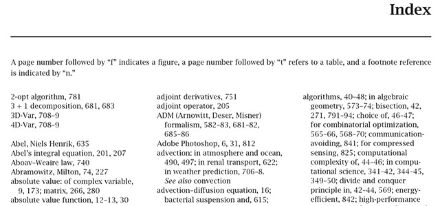
The index was produced by a professional indexer, who made a judgement on which of the many names in the book had significant enough mentions to index. A phrase “Newton’s method” would not generate an index entry for “Newton”, but a phrase describing something that Newton did might.

The index revealed some interesting features. First, there are many entries for famous mathematicians and scientists: 76 in total, ranging from to Niels Henrik Abel to Thomas Young. This means that even though there are no biographical articles, authors have included plenty of historical and biographical snippets. Second, many of the mathematicians might equally well have been mentioned in a book on pure mathematics (Halmos, Poincaré, Smale, Weil), which indicates the blurred boundary between pure and applied mathematics.

A third feature of the index is that the number of locators for the mathematicians and scientists that it contains varies greatly, from 1 to 20. We can use this to produce a highly non-scientific ranking. Here is a Wordle, in which the font size is proportional to the number of times that each name occurs.

wordle-names1.jpg

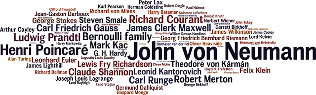
The table of occurrences, which begins

von Neumann, John 20
Poincaré, Henri 12
Bernoulli family 9
Courant, Richard 9
Prandtl, Ludwig 9
Gauss, Carl Friedrich 8
Kac, Mark 8
Maxwell, James Clerk 8
Merton, Robert 8
Runge, Carl 8
Shannon, Claude 8

can be found in this PDF file.

John von Neumann (1903–-1957) emerges as The Companion’s “most mentioned” applied mathematician. Indeed von Neumann was a hugely influential mathematician who contributed to many fields, as his index entry shows:

von Neumann, John: applied mathematics and, 56–59, 73; computational science and, 336–37, 350; economics and, 71, 644, 650, 869; error analysis and, 77; foams and, 740; Monte Carlo method and, 57; random number generation and, 762; shock waves and, 720; spectral theory and, 239–40, 426

von Neumann’s work has strong connections with my own research interests. With Herman Goldstine he published an important rounding error analysis of Gaussian elimination for inverting a symmetric positive definite matrix. He also introduced the alternating projections method that I have used to solve the nearest correlation matrix problem. And he derived important result on unitarily invariant matrix norms and singular value inequalities

More about von Neumann can be found in the biographies

How to Use The Princeton Companion to Applied Mathematics

The Princeton Companion to Applied Mathematics, discussed in these previous posts, has a wide target audience, which includes mathematicians at undergraduate level or above; students, researchers, and professionals in other subjects who use mathematics; and mathematically interested lay readers.

Here are some examples of how different people can use the book.

Maths-research-students-5.jpg

  • Undergraduate students can use it to get an overview of topics they are studying and to find out what areas of applied mathematics they might like to pursue at graduate level. Many of the articles have minimal pre-requisites (indeed some contain few, if any, equations). My article Color Spaces and Digital Imaging, for example, requires just knowledge of integration and basic linear algebra.
  • A teacher might find useful the articles The History of Applied Mathematics and the four-part article Teaching Applied Mathematics, as well as the various short articles on interesting problems and applications (e.g., Cloaking, Bubbles, The Flight of a Golf Ball, Robotics, Medical Imaging, Text Mining, and Voting Systems).
  • Researchers can use the book to find out about topics outside their area that they encounter in seminars but never have the time to study in the research literature.
  • Engineers can use the book to find out about some of the latest mathematical developments relevant to their interests. The articles Aircraft Noise, Inerters, and Signal Processing, and the index entries “aerodynamics”, “energy-efficient buildings”, and “finite-element methods”, are good starting points.
  • Students at all levels can learn about how to read and write mathematics, including the use of relevant computer tools, from several articles in Part VII, “Final Perspectives”.
  • Anyone can use the book for reference. Although it is not a dictionary, encyclopedia, or handbook, The Companion‘s extensive index makes it easy to locate material, including definitions, equations, functions, laws, theorems, and so on.

pcam-index-start.jpg

  • The book, produced with \LaTeX, is a great example of how to typeset mathematics, with examples of all kinds of equations, figures, and tables. For those learning \LaTeX or new to mathematical typesetting it should be a source of ideas and inspiration. The \LaTeX source code is not provided, but feel free to contact me with questions about how things were done and I will write a post that answers the most common questions.
  • The final collection of articles, by mathematicians from China, France, the UK, and the USA, gives advice on how to make the case for mathematics to politicians, and will be of interest to anyone who wishes to promote the importance of mathematics.

The Rise of Mixed Precision Arithmetic

For the last 30 years, most floating point calculations in scientific computing have been carried out in 64-bit IEEE double precision arithmetic, which provides the elementary operations of addition, subtraction, multiplication, and division at a relative accuracy of about 10^{-16}. We are now seeing growing use of mixed precision, in which different floating point precisions are combined in order to deliver a result of the required accuracy at minimal cost.

Single precision arithmetic (32 bits) is an attractive alternative to double precision because it halves the costs of storing and transferring data, and on Intel chips the SSE extensions allow single precision arithmetic to run twice as fast as double.

wpid-qd-compare2.jpg
” /> The Mandelbrot set computed in double and quadruple precision. Image taken from https://www.thasler.com/blog/blog/glsl-part5.

Quadruple precision arithmetic, which was included in the 2008 revision of the IEEE standard, is supported by some compilers, and it can be implemented in terms of double precision arithmetic via double-double arithmetic. Arbitrary precision floating point arithmetic is available through, for example, the GNU MPFR library, the mpmath library for Python, the core data type BigFloat in the new language Julia, VPA arithmetic in the MATLAB Symbolic Math Toolbox, or the Advanpix Multiprecision Computing Toolbox for MATLAB.

Half precision arithmetic, in which a number occupies 16 bits, is supported by the IEEE standard for storage but not for computation. It has been argued that for deep learning half precision, with its relative accuracy of about 10^{-4}
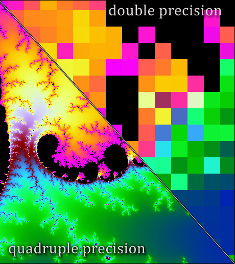
, is good enough for training and running neural networks. Here are some of the ways in which extra precision is currently being used.

  • Iterative refinement, in the traditional form that first became popular in the 1960s, improves the quality of an approximate solution to a linear system via updates obtained from residuals computed in extra precision.
  • When an algorithm suffers instability it may be possible to overcome it by using extra precision in just a few, key places. This has been done recently in eigensolvers and for matrix orthonormalization.
  • Any iterative algorithm that accepts an arbitrary starting point can be run once at a given precision and the solution used to “warm start” a second run of the same algorithm at higher precision. This idea has been used recently in linear programming.
  • Numerical integration of differential equations over long time periods may need higher precision in order to allow the phenomena of interest to be observed. A recent example is in the study of Kerr (rotating) black holes, where the underlying hyperbolic partial differential equation is solved using quadruple precision arithmetic running on GPUs.
  • When one is developing error bounds or testing algorithms, one needs in principle the exact solution. In practice, a solution computed at high precision and rounded to the working precision is usually adequate, and this is an approach I frequently use in my work in numerical linear algebra.

As the relative costs and ease of computing at different precisions evolve, due to changing architectures and software, as well as the disruptive influence of accelerators such as GPUs, we will see an increasing development and use of mixed precision algorithms. In some ways this is analogous to the increasing interoperability of programming languages (illustrated by C++, Julia, and Python, for example): one uses the main tool (precision) one would like to work with and brings in other tools (precisions) as necessary in order to complete the task.

Update: linear programming link updated December 18, 2018.

What is Applied Mathematics For?

Those of us working in applied mathematics are well aware that our field has many important uses in the real world. But if we are put on the spot during a conversation and asked to give some examples it can be difficult to conjure up a convincing list.

One response is to point people to The Princeton Companion to Applied Mathematics. Its 186 articles contains a large number of examples of how applied mathematics is put to work in fields such as sport, engineering, economics, physics, biology, computer science, and finance.

Another way to convince people of the value of applied mathematics is to get them to watch the 1-minute SIAM video below. It was constructed from interviews conducted at a variety of SIAM conferences and comprises snippets of 25 mathematicians saying what they use mathematics for.

Well done to Karthika Swamy Cohen and Michelle Montgomery at SIAM, Adam Bauser and his team at Bauser Media Group, and Sonja Stark at PilotGirl Productions, for producing this great advertisement for applied mathematics!

Top Tips for New LaTeX Users

This article is aimed at relatively new \LaTeX users. It is written particularly for my own students, with the aim of helping them to avoid making common errors. The article exists in two forms: this WordPress blog post and a PDF file generated by \LaTeX, both produced from the same Emacs Org file. Since WordPress does not handle \LaTeX very well I recommend reading the PDF version.

1. New Paragraphs

In \LaTeX a new paragraph is started by leaving a blank line.

Do not start a new paragraph by using \\ (it merely terminates a line). Indeed you should almost never type \\, except within environments such as array, tabular, and so on.

2. Math Mode

Always type mathematics in math mode (as $..$ or \(..\)), to produce “y = f(x)” instead of “y = f(x)”, and “the dimension n” instead of “the dimension n”. For displayed equations use $$, \[..\], or one of the display environments (see Section 7).

Punctuation should appear outside math mode, for inline equations, otherwise the spacing will be incorrect. Here is an example.

  • Correct: The variables $x$, $y$, and $z$ satisfy $x^2 + y^2 = z^2$.
  • Incorrect: The variables $x,$ $y,$ and $z$ satisfy $x^2 + y^2 = z^2.$

For displayed equations, punctuation should appear as part of the display. All equations must be punctuated, as they are part of a sentence.

3. Mathematical Functions in Roman

Mathematical functions should be typeset in roman font. This is done automatically for the many standard mathematical functions that \LaTeX supports, such as \sin, \tan, \exp, \max, etc.

If the function you need is not built into \LaTeX, create your own. The easiest way to do this is to use the amsmath package and type, for example,

\usepackage{amsmath}
...
% In the preamble.
\DeclareMathOperator{\diag}{diag}  
\DeclareMathOperator{\inert}{Inertia}

Alternatively, if you are not using the amsmath package you can type

\def\diag{\mathop{\mathrm{diag}}}

4. Maths Expressions

Ellipses (dots) are never explicitly typed as “…”. Instead they are typed as \dots for baseline dots, as in $x_1,x_2,\dots,x_n$ (giving x_1,x_2,\dots,x_n) or as \cdots for vertically centered dots, as in $x_1 + x_2 + \cdots + x_n$ (giving x_1 + x_2 + \cdots + x_n).

Type $i$th instead of $i'th$ or $i^{th}$. (For some subtle aspects of the use of ellipses, see How To Typeset an Ellipsis in a Mathematical Expression.)

Avoid using \frac to produce stacked fractions in the text. Write n^3/3 flops instead of \frac{n^3}{3} flops.

For “much less than”, type \ll, giving \ll, not <<, which gives <<. Similarly, “much greater than” is typed as \gg, giving \gg. If you are using angle brackets to denote an inner product use \langle and \rangle:

  • incorrect: <x,y>, typed as $<x,y>$.
  • correct: \langle x,y \rangle, typed as $\langle x,y \rangle$

5. Text in Displayed Equations

When a displayed equation contains text such as “subject to x \ge 0”, instead of putting the text in \mathrm put the text in an \mbox, as in \mbox{subject to $x \ge 0$}. Note that \mbox switches out of math mode, and this has the advantage of ensuring the correct spacing between words. If you are using the amsmath package you can use the \text command instead of \mbox.

Example

$$
      \min\{\, \|A-X\|_F: \mbox{$X$ is a correlation matrix} \,\}.
$$

6. BibTeX

Produce your bibliographies using BibTeX, creating your own bib file. Note three important points.

  • “Export citation” options on journal websites rarely produce perfect bib entries. More often than not the entry has an improperly cased title, an incomplete or incorrectly accented author name, improperly typeset maths in the title, or some other error, so always check and improve the entry.
  • If you wish to cite one of my papers download the latest version of njhigham.bib (along with strings.bib supplied with it) and include it in your \bibliography command.
  • Decide on a consistent format for your bib entry keys and stick to it. In the format used in the Numerical Linear Algebra group at Manchester a 2010 paper by Smith and Jones has key smjo10, a 1974 book by Aho, Hopcroft, and Ullman has key ahu74, while a 1990 book by Smith has key smit90.

7. Spelling Errors and \LaTeX Errors

There is no excuse for your writing to contain spelling errors, given the wide availability of spell checkers. You’ll need a spell checker that understands \LaTeX syntax.

There are also tools for checking \LaTeX syntax. One that comes with TeX Live is lacheck, which describes itself as “a consistency checker for LaTeX documents”. Such a tool can point out possible syntax errors, or semantic errors such as unmatched parentheses, and warn of common mistakes.

8. Quotation Marks

\LaTeX has a left quotation mark, denoted here \lq, and a right quotation mark, denoted here \rq, typed as the single left and right quotes on the keyboard, respectively. A left or right double quotation mark is produced by typing two single quotes of the appropriate type. The double quotation mark always itself produces the same as two right quotation marks. Example: ``hello'' is typed as \lq\lq hello \rq\rq.

9. Captions

Captions go above tables but below figures. So put the caption command at the start of a table environment but at the end of a figure environment. The \label statement should go after the \caption statement (or it can be put inside it), otherwise references to that label will refer to the subsection in which the label appears rather than the figure or table.

10. Tables

\LaTeX makes it easy to put many rules, some of them double, in and around a table, using \cline, \hline, and the | column formatting symbol. However, it is good style to minimize the number of rules. A common task for journal copy editors is to remove rules from tables in submitted manuscripts.

11. Source Code

\LaTeX source code should be laid out so that it is readable, in order to aid editing and debugging, to help you to understand the code when you return to it after a break, and to aid collaborative writing. Readability means that logical structure should be apparent, in the same way as when indentation is used in writing a computer program. In particular, it is is a good idea to start new sentences on new lines, which makes it easier to cut and paste them during editing, and also makes a diff of two versions of the file more readable.

Example:

Good:

$$
U(\zbar) = U(-z) = 
            \begin{cases}
                -U(z),   & z\in D, \\ 
                -U(z)-1, & \mbox{otherwise}.
            \end{cases}
$$

Bad:

$$U(\zbar) = U(-z) = 
\begin{cases}-U(z),   & z\in D, \\ 
-U(z)-1, & \mbox{otherwise}.
\end{cases}$$

12. Multiline Displayed Equations

For displayed equations occupying more than one line it is best to use the environments provided by the amsmath package. Of these, align (and align* if equation numbers are not wanted) is the one I use almost all the time. Example:

\begin{align*}
  \cos(A) &= I - \frac{A^2}{2!} + \frac{A^4}{4!} + \cdots,\\
  \sin(A) &= A - \frac{A^3}{3!} + \frac{A^5}{5!} -  \cdots,
\end{align*}

Others, such as gather and aligned, are occasionally needed.

Avoid using the standard \LaTeX environment eqnarray, because it doesn’t produce as good results as the amsmath environments, nor is it as versatile. For more details see the article Avoid Eqnarray.

13. Synonyms

This final category concerns synonyms and is a matter of personal preference. I prefer \ge and \le to the equivalent \geq \leq\ (why type the extra characters?).

I also prefer to use $..$ for math mode instead of \(..\) and $$..$$ for display math mode instead of \[..\]. My preferences are the original \TeX syntax, while the alternatives were introduced by \LaTeX. The slashed forms are obviously easier to parse, but this is one case where I prefer to stick with tradition. If dollar signs are good enough for Don Knuth, they are good enough for me!

I don’t think many people use \LaTeX‘s verbose

\begin{math}..\end{math}

or

\begin{displaymath}..\end{displaymath}

Also note that \begin{equation*}..\end{equation*} (for unnumbered equations) exists in the amsmath package but not in in \LaTeX itself.

Programming Languages: An Applied Mathematics View

prog-langs.jpg

A lot of applied mathematics relies on computation, whether symbolic or numeric, so many applied mathematicians need to program as part of their work. It was therefore natural to include an article on programming languages in The Princeton Companion to Applied Mathematics.

The article, which I wrote, has two main purposes. The first is to give a history of those programming languages relevant to applied mathematics. The first such language, and indeed the first high-level programming language, was Fortran (1957). The language was standardized in 1966 and it is still going strong, with the most recent standard published in 2008. Developments in programming languages show no sign of abating, with the introduction in recent years of new languages such as Scala (2003), Clojure (2007, a dialect of Lisp), and Julia (2012), as well as new standards for older languages such as C (2011) and C++ (2011).

The second purpose of the article is to discuss mathematical aspects of programming, including

  • notation (infix, prefix, reverse-Polish)
  • implementation of complex arithmetic
  • floating-point semantics
  • high-precision computations
  • types
  • complexity analysis of codes
  • structured programming
  • literate programming
  • domain-specific languages

One issue that I discuss is the mutually beneficial influences that mathematics and programming languages have had on each other. For example, the notation for the ceiling and floor functions that map a real number to the next larger or smaller integer, respectively, illustrated by \lceil 4.3 \rceil = 5 and \lfloor 4.3 \rfloor = 4, was first introduced in the programming language APL. The colon notation for array subscripting, A(i:j,r:s), used in Algol 68 and MATLAB, is now routinely used in linear algebra, in both equations and in pseudocode.

On the other hand, mathematics has influenced, or anticipated, syntax in programming languages. In the 1800s Cayley proposed two different notations to distinguish between the products AB^{-1} and B^{-1}A in the context of groups, but both were ungainly and difficult to typeset. In 1928, Hensel suggested the notation A/B and B\backslash A. Although his suggestion appears to have attracted little or no attention, it was was reinvented by Cleve Moler for MATLAB and is now a notation familiar to anyone who works in numerical linear algebra.

At the start of the article I include a figure containing the first program written for a stored-program computer, namely the highest factor routine that ran on the Manchester “Baby” on June 21, 1948. The program was by Tom Kilburn and is taken from Geoff Tootill‘s notebook. Tootill is still alive (aged 93), and he kindly gave permission for me to reproduce the image.

The article, which has the same title as this post, can be downloaded in pre-publication form as an EPrint.

Wobbly Tables

In The Princeton Companion to Applied Mathematics (page 50) I mention that a four-legged table provides an example of an ill-posed problem. If we take a table having four legs of equal length lying on a flat surface and shorten one leg by an arbitrarily small amount then the weight supported by that leg will jump from one quarter of the total weight to zero.

150912-1434-19-6791.jpg

A table with one leg shorter than the others wobbles, as may one sitting on an uneven floor, and how to cure wobbly tables has been the subject of a number of papers over the years. The tongue-in cheek article

Hanspeter Kraft, The Wobbly Garden Table, Journal of Biological Physics and Chemistry 1, 95-96, 2001

describes how an engineer, a physicist, and a mathematician would go about solving the problem. The engineer would invent an adjustable leg. The physicist would submit a research proposal to tackle the more general problem of “the stability of multiply-legged objects on rough surfaces”. The mathematician would construct an argument based on the intermediate value theorem to show that stability can be restored with a suitable rotation of no more than 90 degrees. This argument has been discussed by several authors, but turning it into a mathematically precise statement with appropriate assumptions on the table and the ground on which it rests is not easy.

The two most recent contributions to this topic that I am aware of are

A. Martin, On the Stability of Four-Legged Tables, Physics Letters A, 360, 495-500, 2007

Bill Baritompa, Rainer Löwen, Burkard Polster, and Marty Ross, Mathematical Table Turning Revisited, arXiv:math/0511490v1, 17 pp., 2008

In the latter paper it is shown that if the ground on which a rectangular table rests slopes by less than 35.36 degrees and the legs of the table are at least half as long as its diagonals then the rotation trick works.

For more insight into this problem you may like to watch the video below in which Matthias Kreck explains the problem with the aid of some excellent animations.

Mathematics in Color

circle-rgb.jpg

Color is a fascinating subject. Important early contributions to our understanding of it came from physicists and mathematicians such as Newton, Young, Grassmann, Maxwell, and Helmholtz. Today, the science of color measurement and description is well established and we rely on it in our daily lives, from when we view images on a computer screen to when we order paint, wallpaper, or a car, of a specified color.

For practical purposes color space, as perceived by humans, is three-dimensional, because our retinas have three different types of cones, which have peak sensitivities at wavelengths corresponding roughly to red, green, and blue. It’s therefore possible to use linear algebra in three dimensions to analyze various aspects of color.

Metamerism

A good example of the use of linear algebra is to understand metamerism, which is the phenomenon whereby two objects can appear to have the same color but are actually giving off light having different spectral decompositions. This is something we are usually unaware of, but it is welcome in that color output systems (such as televisions and computer monitors) rely on it.

Mathematically, the response of the cones on the retina to light can be modeled as a matrix-vector product Af, where A is a 3-by-n matrix and f is an n-vector that contains samples of the spectral distribution of the light hitting the retina. The parameter n is a discretization parameter that is typically about 80 in practice. Metamerism corresponds to the fact that Af_1 = Af_2 is possible for different vectors f_1 and f_2. This equation is equivalent to saying that Ag = 0 for a nonzero vector g = f_1-f_2, or, in other words, that a matrix with fewer rows than columns has a nontrivial null space.

Metamerism is not always welcome. If you have ever printed your photographs on an inkjet printer you may have observed that a print that looked fine when viewed indoors under tungsten lighting can have a color cast when viewed in daylight.

LAB Space: Separating Color from Luminosity

In digital imaging the term channel refers to the grayscale image representing the values of the pixels in one of the coordinates, most often R, G, or B (for red, green, and blue) in an RGB image. It is sometimes said that an image has ten channels. The number ten is arrived at by combining coordinates from the representation of an image in three different color spaces. RGB supplies three channels, a space called LAB (pronounced “ell-A-B”) provides another three channels, and the last four channels are from CMYK (cyan, magenta, yellow, black), the color space in which all printing is done.

LAB is a rather esoteric color space that separates luminosity (or lightness, the L coordinate) from color (the A and B coordinates). In recent years photographers have realized that LAB can be very useful for image manipulations, allowing certain things to be done much more easily than in RGB. This usage is an example of a technique used all the time by mathematicians: if we can’t solve a problem in a given form then we transform it into another representation of the problem that we can solve.

As an example of the power of LAB space, consider this image of aeroplanes at Schiphol airport.

060721-1320-30-8896-org.jpg
Original image.

Suppose that KLM are considering changing their livery from blue to pink. How can the image be edited to illustrate how the new livery would look? “Painting in” the new color over the old using the brush tool in image editing software would be a painstaking task (note the many windows to paint around and the darker blue in the shadow area under the tail). The next image was produced in just a few seconds.

060721-1320-30-8896-lab.jpg
Image converted to LAB space and A channel flipped.

How was it done? The image was converted from RGB to LAB space (which is a nonlinear transformation) and then the coordinates of the A channel were replaced by their negatives. Why did this work? The A channel represents color on a green–magenta axis (and the B channel on a blue–yellow axis). Apart from the blue fuselage, most pixels have a small A component, so reversing the sign of this component doesn’t make much difference to them. But for the blue, which has a negative A component, this flipping of the A channel adds just enough magenta to make the planes pink.

You may recall from earlier this year the infamous photo of a dress that generated a huge amount of interest on the web because some viewers perceived the dress as being blue and black while others saw it as white and gold. A recent paper What Can We Learn from a Dress with Ambiguous Colors? analyzes both the photo and the original dress using LAB coordinates. One reason for using LAB in this context is its device independence, which contrasts with RGB, for which the coordinates have no universally agreed meaning.

The Princeton Companion to Applied Mathematics

My article Color Spaces and Digital Imaging in The Princeton Companion to Applied Mathematics gives an introduction to the mathematics of color and the representation and manipulation of digital images. In particular, it emphasizes the role of linear algebra in modeling color and gives more detail on LAB space.

I have one update to the article. Since the book went to press a second edition of the book that I cite by Dan Margulis, Photoshop LAB Color: The Canyon Conundrum And Other Adventures In The Most Powerful Colorspace, has appeared (amazon.com and amazon.co.uk). I do not yet have the book but it appears to have a number of improvements on the excellent first edition.

Finally, in the article I mention the problem of finding good color maps and the problems with the commonly used rainbow color map. For a nicely illustrated talk on this topic see Perceptual Color Maps in matplotlib for Oceanography given at SciPy 2015 by Kristen Thyng.

University-of-Manchester-Maths-059.jpg
The author speaking about rainbow color maps at a UoM School of Mathematics Alumni Event at The Royal Institution, London. Photo: Chris Mann Photography.

Knuth on Knowing Your Audience

Donald Knuth has a great ability to summarize things in pithy, quotable nuggets. A good example is the following sentence from his 2001 book Things a Computer Scientist Rarely Talks About:

The amount of terror that lives in a speaker’s stomach when giving a lecture is proportional to the square of the amount he doesn’t know about his audience.

Knuth’s point is about preparation, and it brings to mind the words of Benjamin Franklin, “By failing to prepare, you are preparing to fail”.

It’s essential to find out as much as possible about your audience, not just so that you feel more confident, but also so that what you deliver is appropriate for that audience.

As academics we are used to giving seminars and conference talks for which we know that the audience will be made up of peers, and we usually just need to ascertain where to aim the talk on the axes general researcher–specialist and graduate student–experienced researcher.

For any other talk it is important to go to some effort to find out who will be in the audience, perhaps asking for a list of attendees if the event requires registration. For an after-dinner talk you may want to know whether certain key people who you are thinking of mentioning will be in the audience. For a talk to a general audience you will want to assess the base level of technical knowledge that can be assumed.

Keep these thoughts in mind when that sought-after invitation to give a “TED talk” arrives in your mailbox.

ted-talk.jpg
©Guy Venables. http://www.guyscartoons.com. Used with permission.

Anderson Acceleration

Anderson acceleration, also known in quantum chemistry as Pulay mixing or direct inversion in the iterative subspace (DIIS), is a technique for accelerating the convergence of a fixed-point iteration. It has been widely used in electronic structure computations, but does not seem to be well known to numerical analysts.

Anderson’s original paper is from 1965 and is well cited, as Google Scholar shows: and65-gs.jpg 
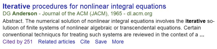
I learned about Anderson acceleration in the minisymposium Anderson Acceleration and Applications organized by Tim Kelley at the SIAM Conference on Computational Science and Engineering in Salt Lake City in March 2015. Tim gave an excellent overview of the topic in the opening talk. The slides for that talk are available on Tim’s website.

PhD student Nataša Strabić and I have shown that Anderson acceleration works very well for speeding up the alternating projections method for computing the nearest correlation matrix. It typically gives a reduction in the number of iterations by a factor at least 2 for the standard nearest correlation matrix problem and by at least a factor 3 when additional constraints are imposed on the matrix (specified elements fixed and a lower bound on the smallest eigenvalue). In some cases the reduction is by a factor of as much as 25. Since the overhead of Anderson acceleration is small, significant speedups are obtained.

In my 2013 post The Nearest Correlation Matrix I included a MATLAB code nearcorr.m. In place of this I now recommend our new accelerated code nearcorr_aa.m, which is available from the repository anderson-accel-ncm on GitHub. Our paper describing this work is available on MIMS EPrints.

For me this project is an excellent illustration of the importance of going to conferences in order to learn of new ideas and new developments.