Sixty years ago James Wilkinson published his backward error analysis of Gaussian elimination for solving a linear system 


where 


where the 


With partial pivoting, in which row interchanges are used to ensure that at each stage the pivot element is the largest in its column, Wilkinson showed that 
It is easy to experiment with growth factors in MATLAB. I will use the function
function g = gf(A)
%GF     Approximate growth factor.
%   g = GF(A) is an approximation to the
%   growth factor for LU factorization
%   with partial pivoting.
[~,U] = lu(A);
g = max(abs(U),[],'all')/max(abs(A),[],'all');
It computes a lower bound on the growth factor (since it only considers 
>> rng(1); n = 10000; gf(randn(n))
ans =
6.1335e+01
Growth of 61 is unremarkable for a matrix of this size. Now we try a matrix of the same size generated by the gallery('randsvd') function:
>> A = gallery('randsvd',n,1e6,2,[],[],1);
>> gf(A)
ans =
9.7544e+02
This function generates an 1e6 specifies the 2-norm condition number, while the 2 (the mode parameter) specifies that there is only one small singular value, so the singular values are 1 repeated 
It turns out that mode 2 randsvd matrices generate with high probability growth factors of size at least 
>> gf(A(:,randperm(n)))
ans =
7.8395e+02
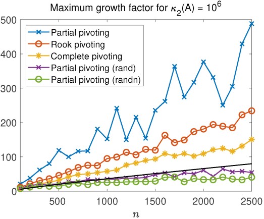
Here is a plot showing the maximum over 12 randsvd matrices for each 
rand and randn matrices. The black curve is
What is the explanation for this large growth? It stems from three facts.
- Haar distributed orthogonal matrices have the property that that their elements are fairly small with high probability, as shown by Jiang in 2005.
- If the largest entries in magnitude of
are both small, in the sense that their product is
, then
for any pivoting strategy. This was proved by Des Higham and I in the paper Large Growth Factors in Gaussian Elimination with Pivoting.
- If
is an orthogonal matrix generating large growth then a rank-1 perturbation of 2-norm at most 1 tends to preserve the large growth.
For full details see the new EPrint Random Matrices Generating Large Growth in LU Factorization with Pivoting by Des Higham, Srikara Pranesh and me.
Is growth of order
- The largest dense linear systems
. If we work in single precision then
and so LU factorization can potentially be completely unstable if there is growth of order
- For IEEE half precision arithmetic growth of order
. It was overflow in half precision LU factorization on randsvd matrices that alerted us to the large growth.

It is theoretically possible, but unlikely, that large growth is present at the k-th step of the elimination for k < n, but disappears from U. Have you ever looked for this? (I haven't.)
Good point, Cleve. I don’t think this is an issue as regards very large growth – see the note at https://nickhigham.files.wordpress.com/2020/06/note_rhonest.pdf
Hi Nick, I know there is some work showing that a random matrix or a randomly perturbed matrix has nice condition number (the latter falls into the umbrella of ‘smoothed analysis’). Is there any work along these lines for the growth factor?
Yes: see “Smoothed Analysis of the Condition Numbers and Growth Factors of Matrices” https://doi.org/10.1137/S0895479803436202